Year 2023
This page groups the 2023 graphs.
Scatter representation
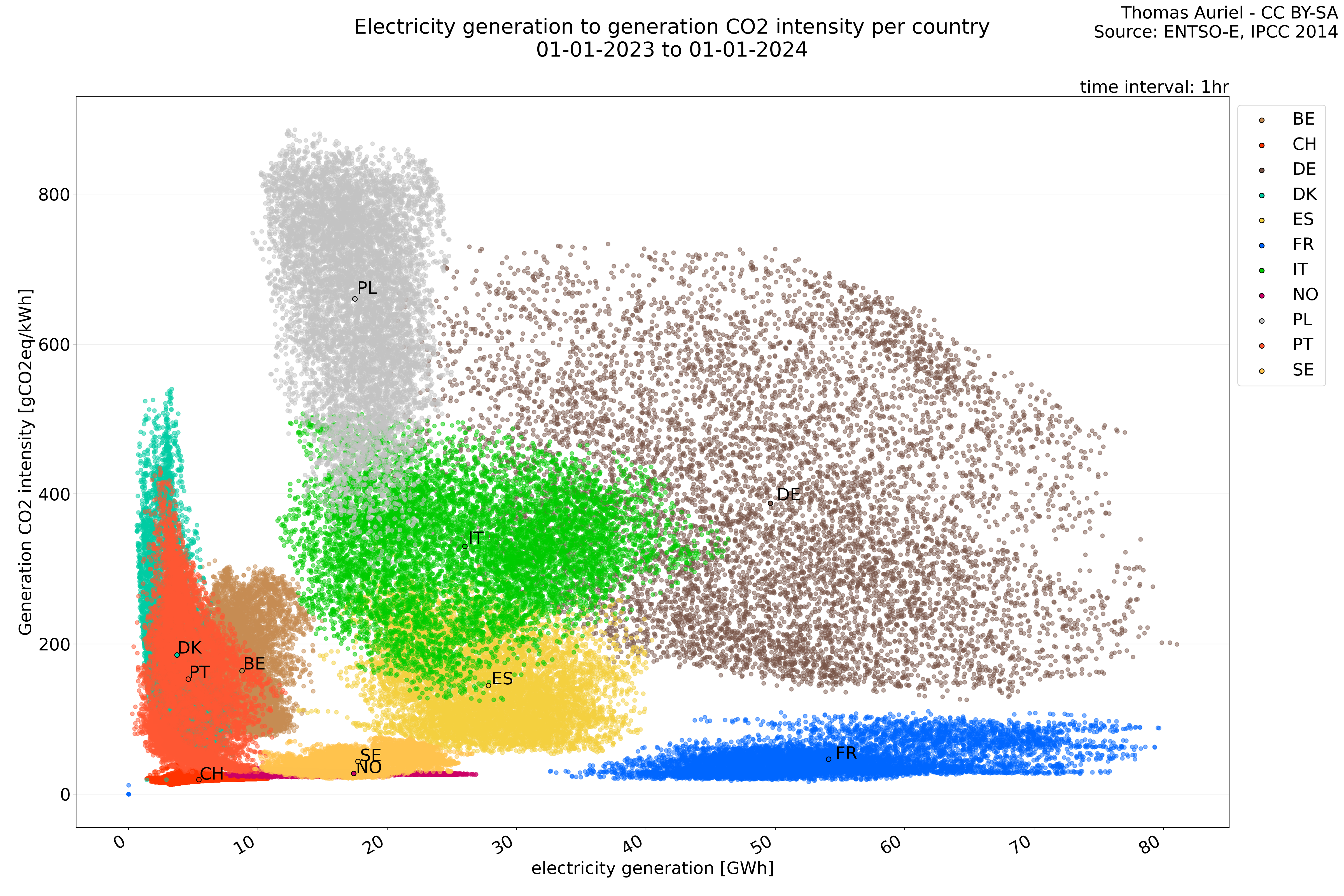
Scatter plots are a common type of graph used to visualize the relationship between two variables. In a scatter plot, each point represents a data pair. For the scatter plot in question, the horizontal axis (x-axis) represents one hour of production, while the vertical axis (y-axis) shows the CO2 intensity for the same hour. Each point on the graph correlates an hour of production with its corresponding CO2 intensity.
One of the key features of scatter plots is the use of color to differentiate between groups. In this scatter plot, each color represents a different country, allowing viewers to easily distinguish the data for each nation. This is particularly useful when comparing trends or patterns between different countries.
To read the scatter plot, locate a point on the graph and trace it back to both axes. The x-axis value gives the hour of production, and the y-axis value gives the CO2 intensity for that hour. By examining where the points are clustered, you can identify trends. For example, a cluster of points towards the lower right might indicate that higher production hours are associated with lower CO2 intensity for a particular country.
Scatter plots can also reveal outliers - points that do not fit the general pattern. These can be critical for identifying exceptional cases or errors in data.
This scatter plot provides a visual representation that can help in understanding how production levels relate to CO2 emissions across different countries. It is an invaluable tool for identifying patterns, trends, and outliers in data, making complex information more accessible and easier to understand.
Production
The generation plots exclusively considers national power plants.
Consumption
The consumption graph employs the method at describe in this blog post. It plots consumers' electricity usage, helping analyze consumption impact.
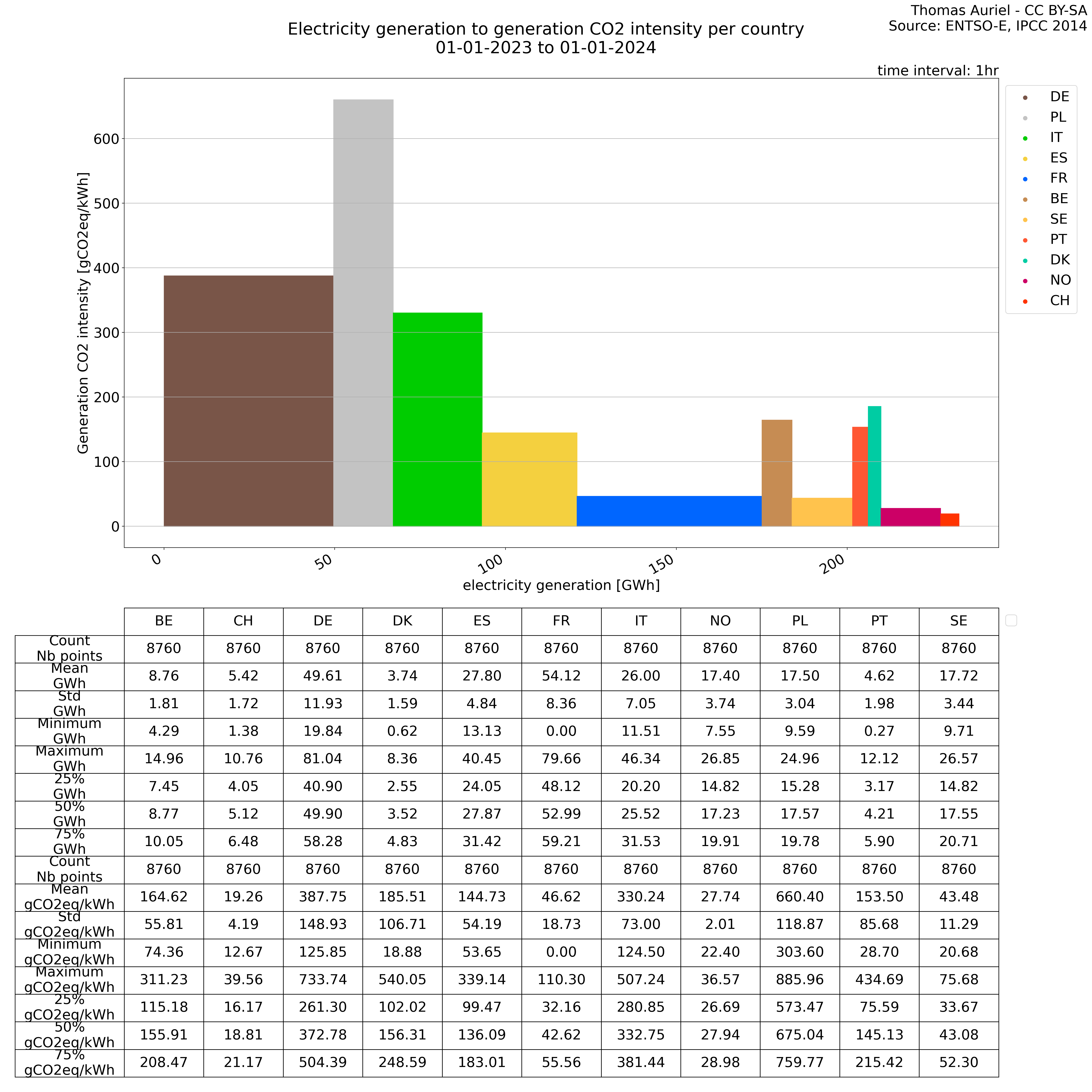
Square representation
Square plots are a specialized type of graph utilized for visualizing complex data relationships. In the specific square plot under discussion, each square represents a country, distinguished by unique colors. This plot is designed to compare two key variables: average production and average CO2 intensity, across a range of countries.
In these square plots, the horizontal axis (x-axis) signifies the average production, while the vertical axis (y-axis) corresponds to the average CO2 intensity. The positioning of each square is dictated by these two metrics. Unlike scatter plots where points are independently placed, in square plots, squares are arranged adjacently, forming a continuous line. Consequently, the x-axis also functions as a cumulative representation of the squares, aggregating the data visually.
An essential feature of the square plot is the size of each square, which is proportional to the total CO2 emissions of the represented country, calculated by multiplying CO2 intensity with production. Larger squares indicate higher emissions.
Interpreting the square plot involves examining the position and size of each square. Horizontal positioning reflects average production, and vertical positioning indicates average CO2 intensity. The size of a square provides a visual indicator of the country's total CO2 emissions. The squares are organized by size, with the largest emitters positioned on the left side of the plot.
Such graphs are particularly effective in showcasing and comparing the environmental impacts of different countries, considering their production levels and CO2 intensity. They offer a clear, visual means to identify major emitters and to compare them in terms of production efficiency and environmental footprint.
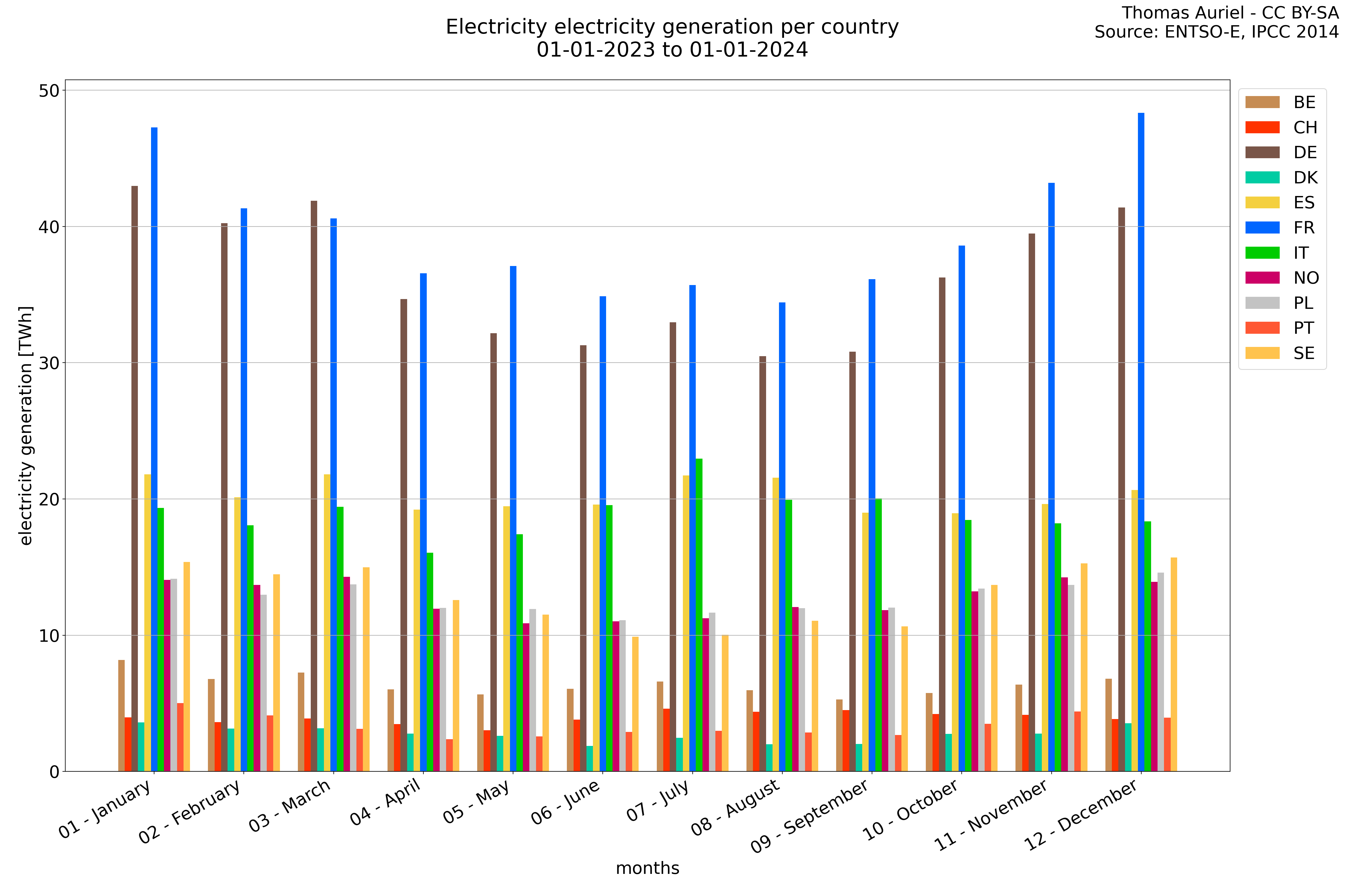
Production
The generation plots exclusively considers national power plants.
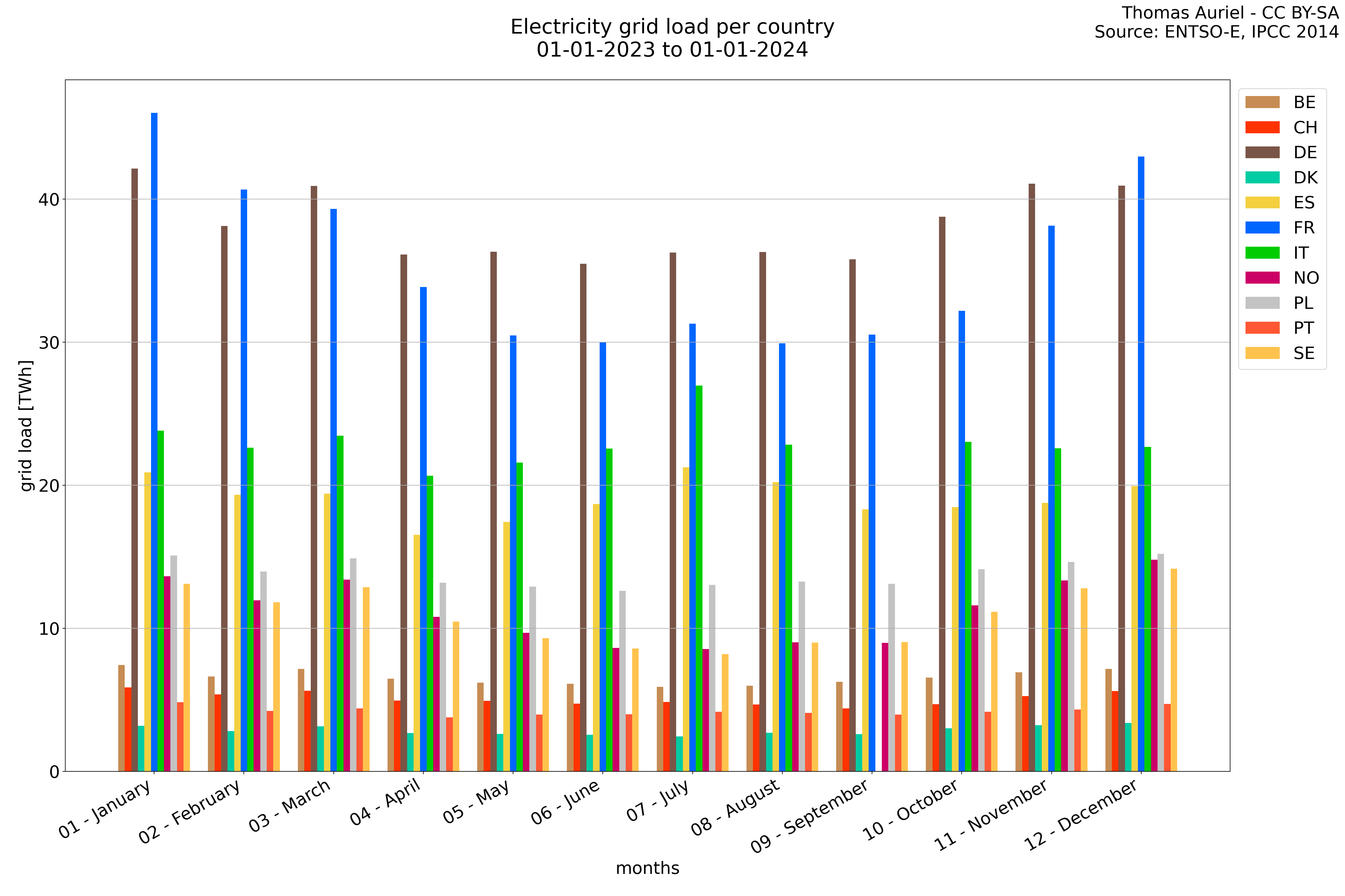
Consumption
The consumption graph employs the method at describe in this blog post. It plots consumers' electricity usage, helping analyze consumption impact
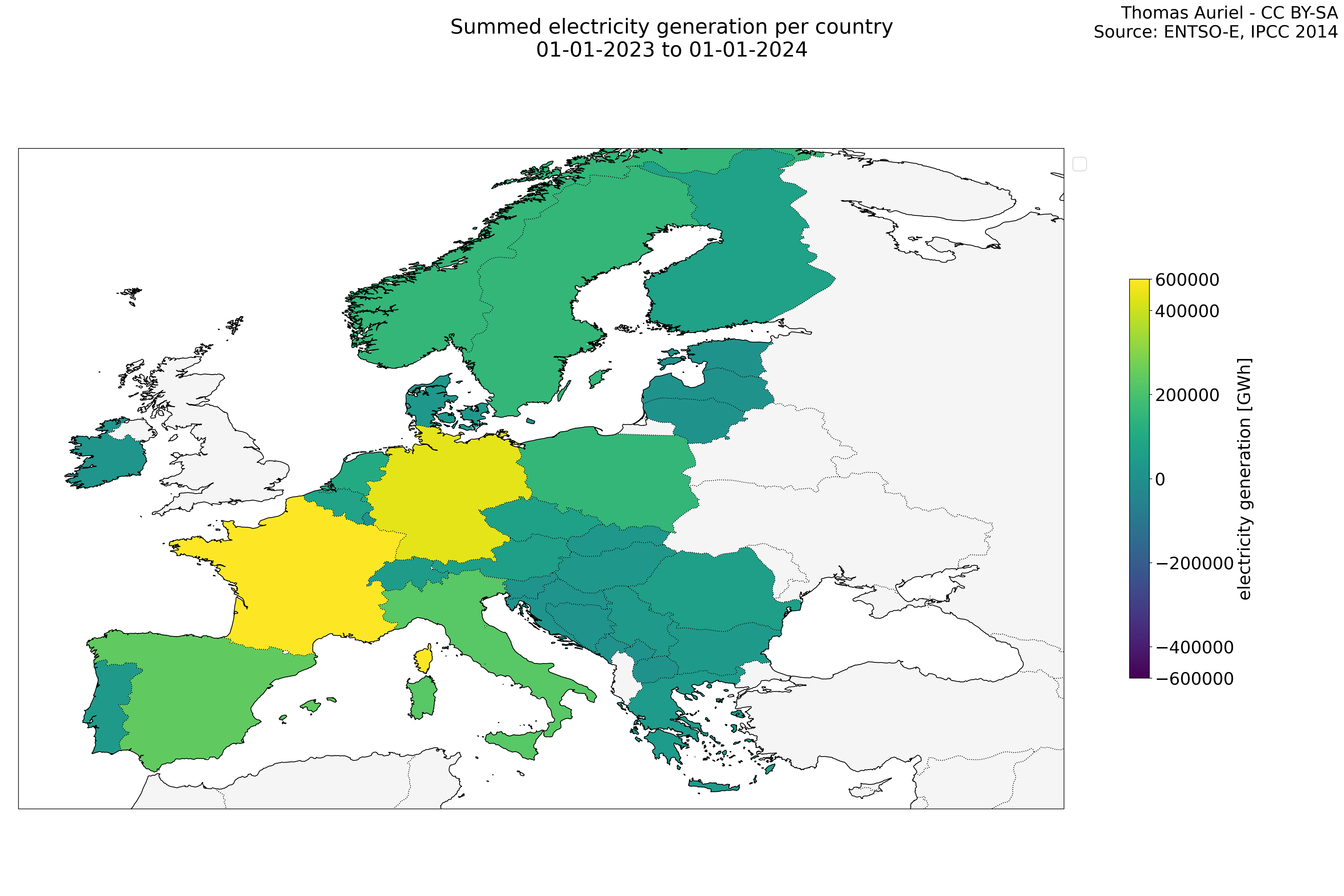
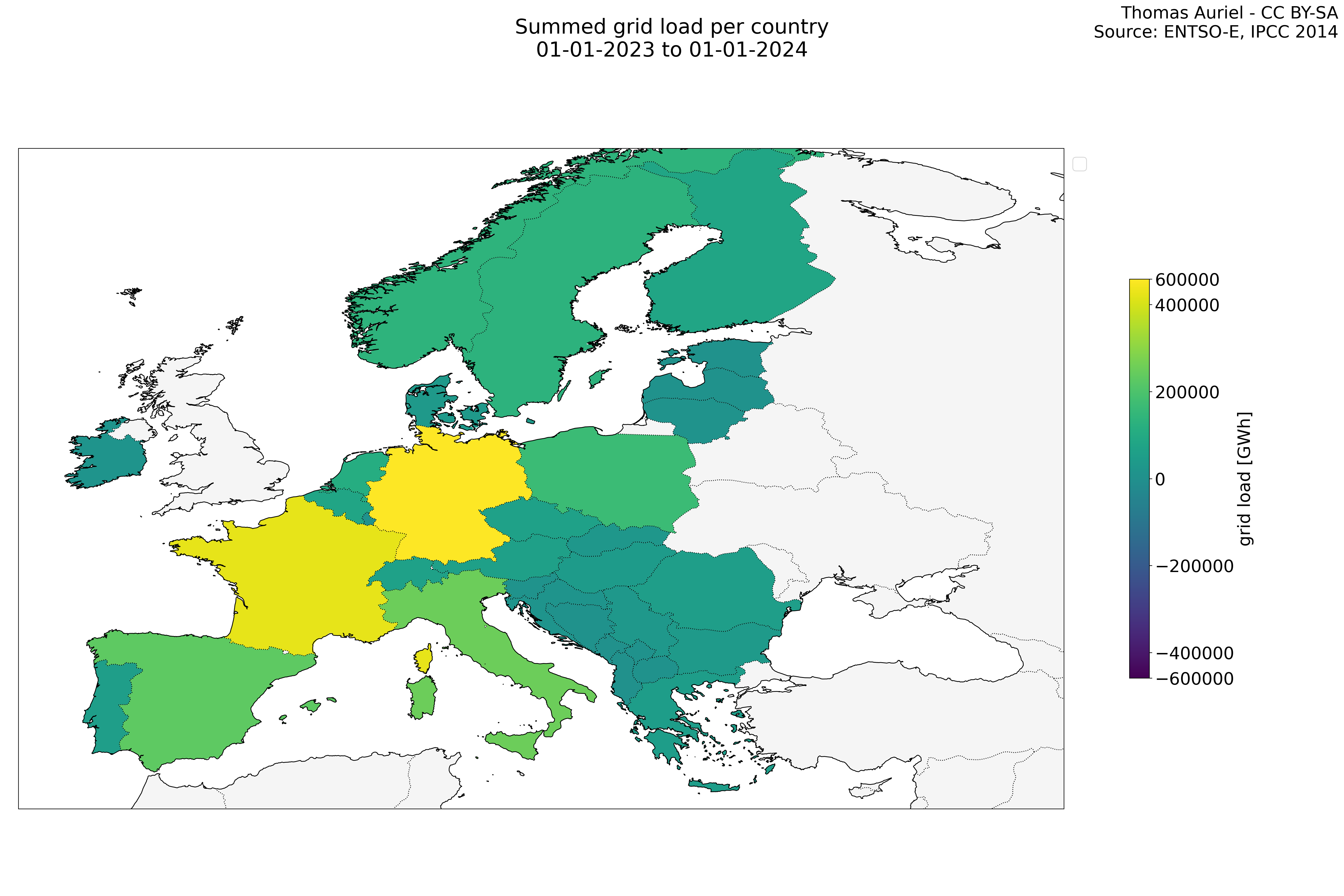
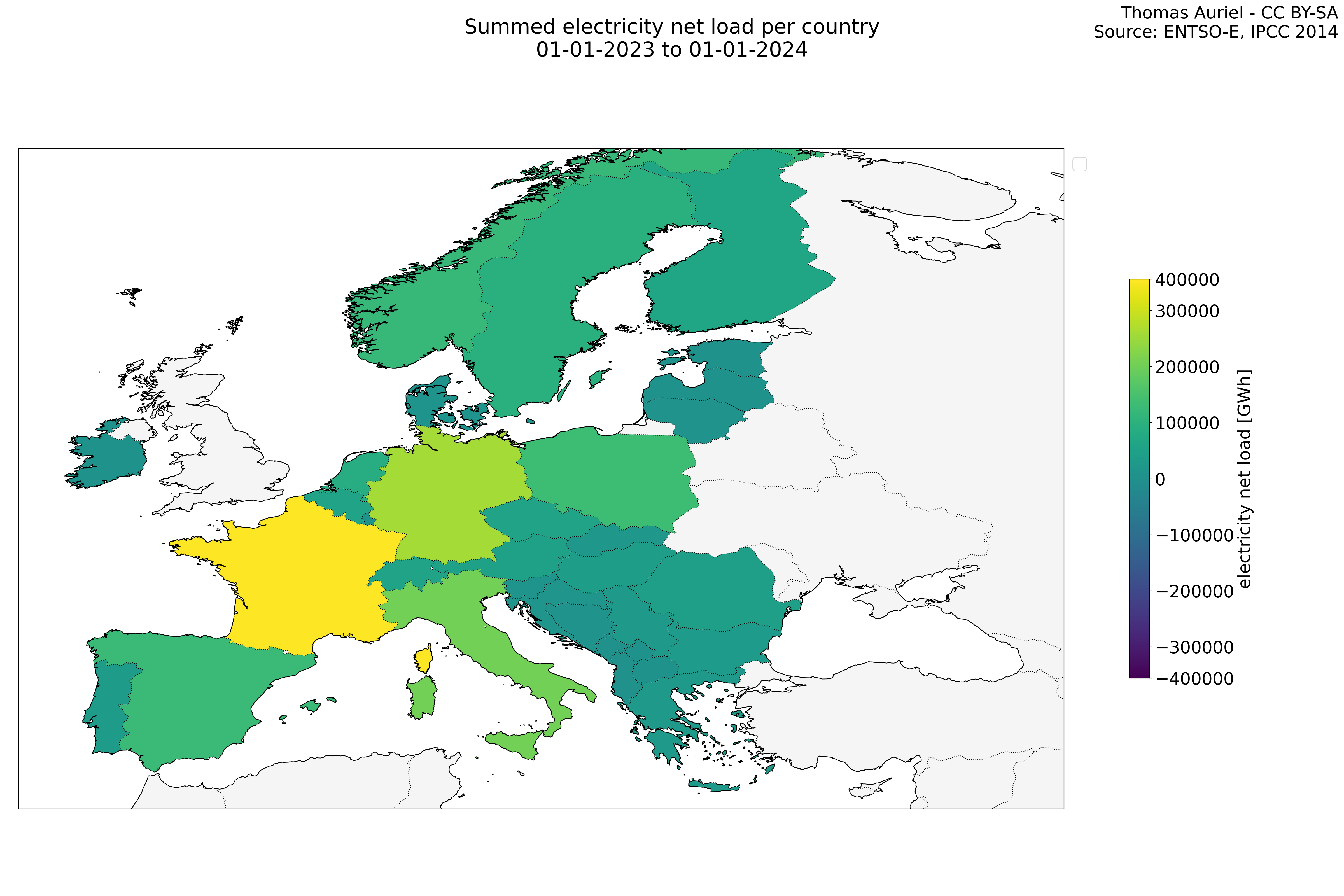
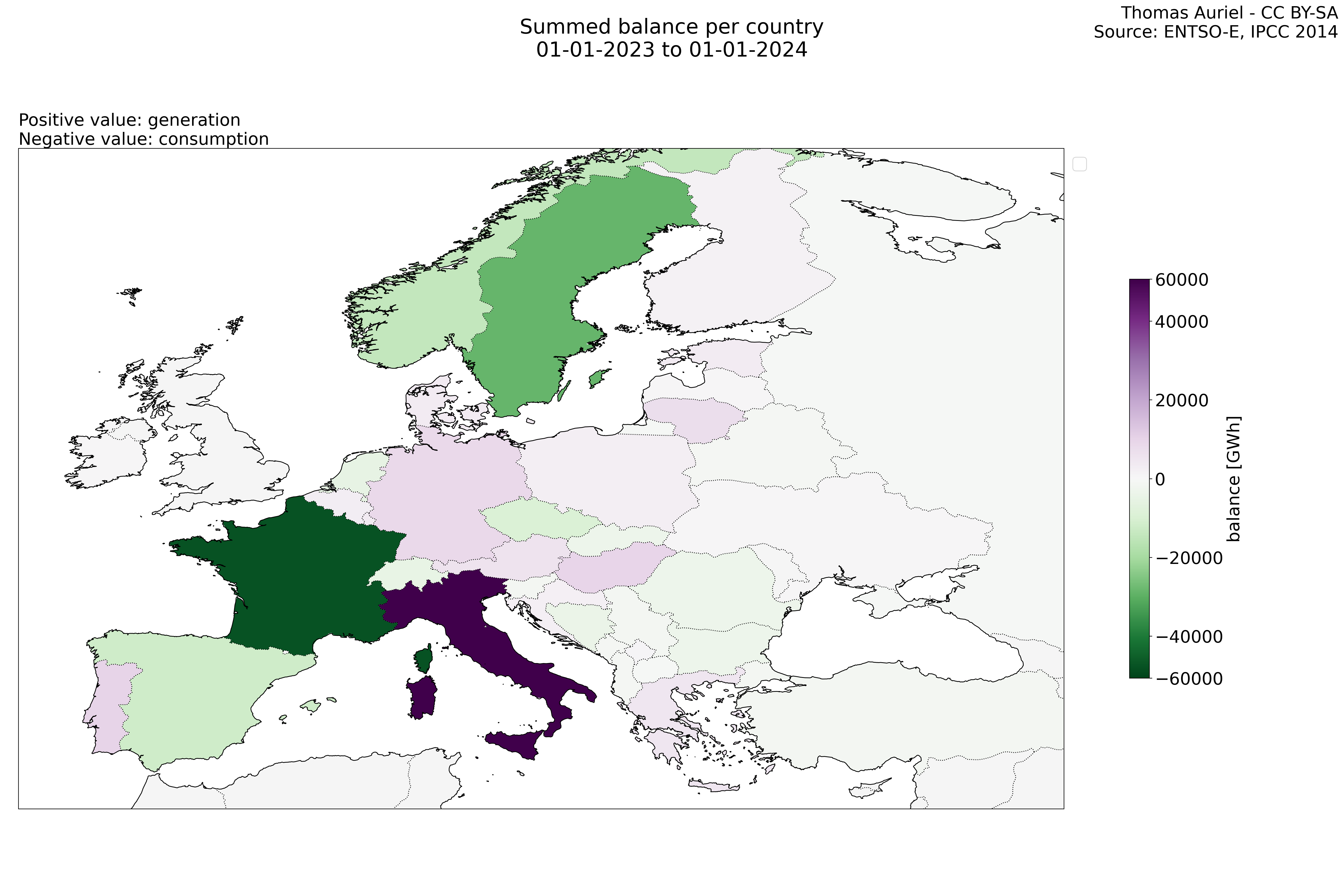
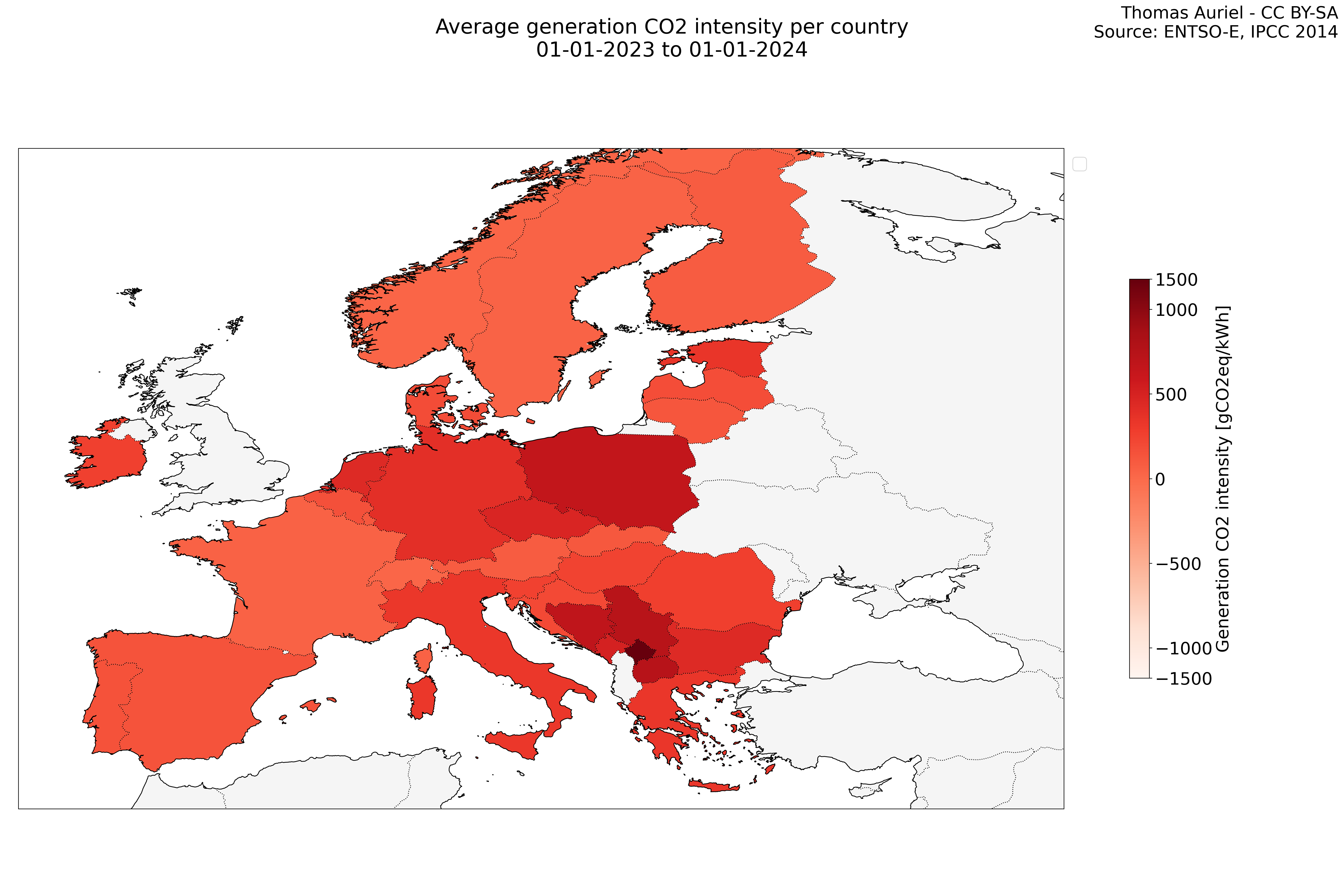
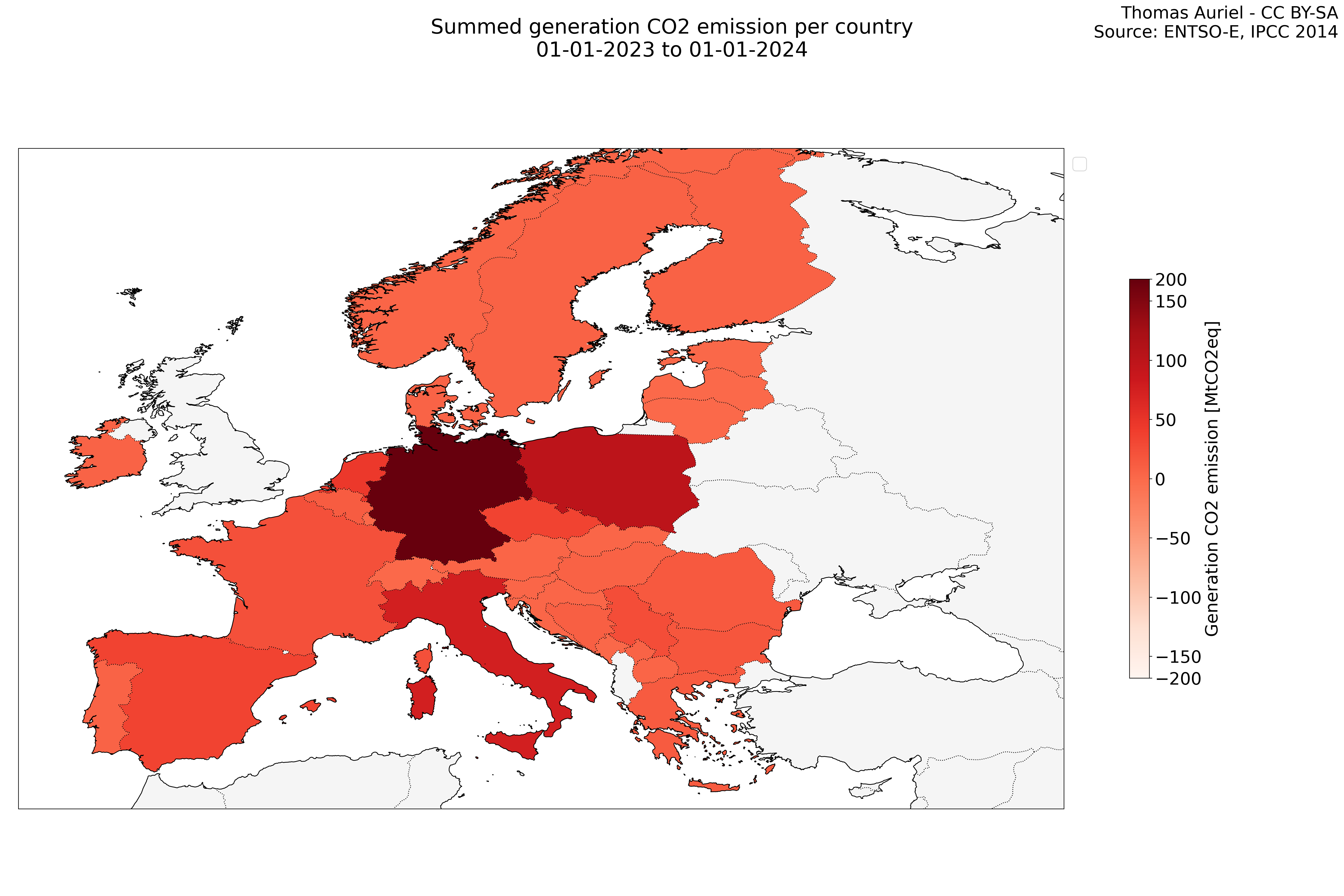
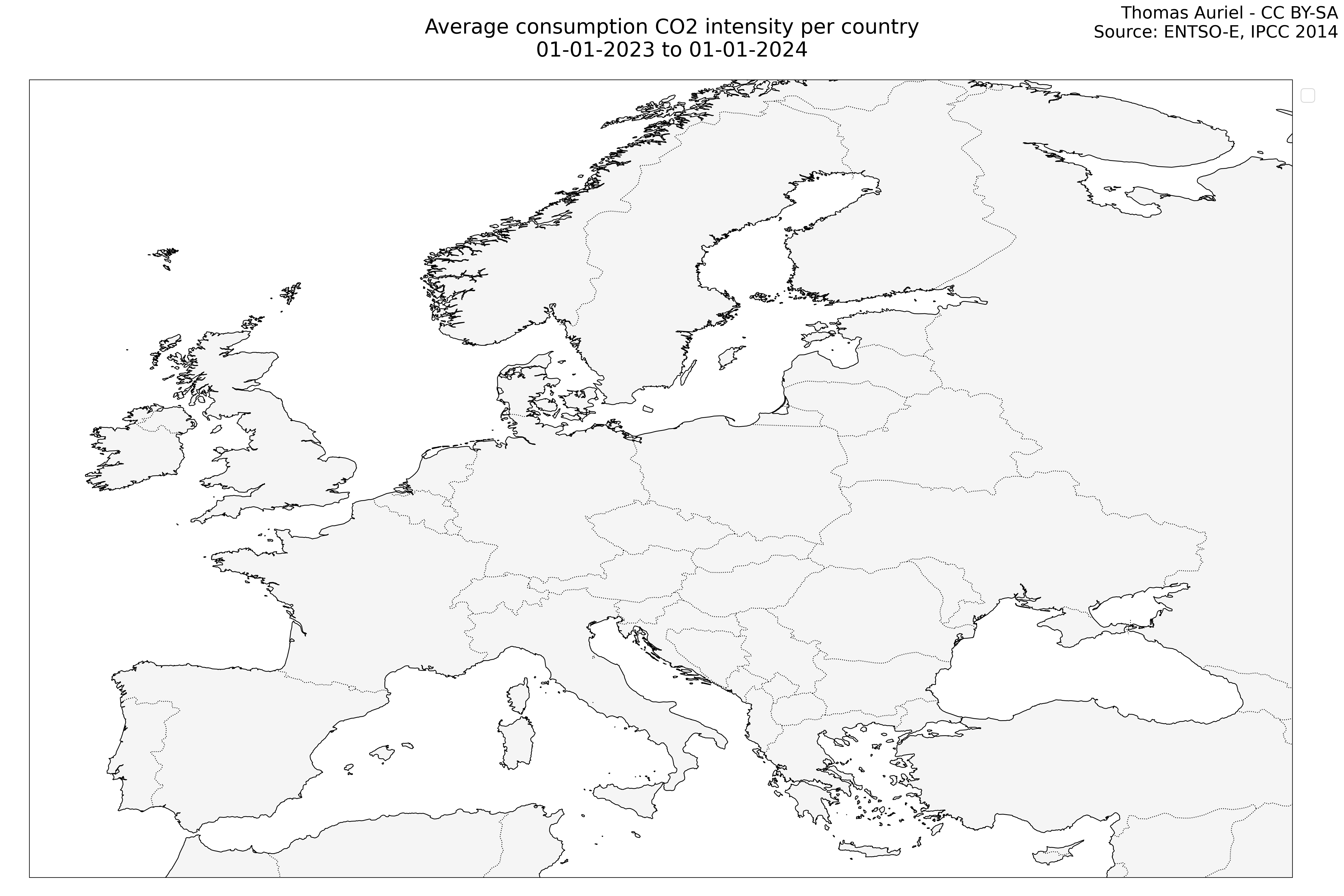
Map representation
Map plots display data on a map where each country is distinct. Depending on the variable, values are either summed or averaged. Summation maps accumulate data, making larger countries more prominent, while averaging maps use shading to represent average values within each country. These plots provide a visual representation of geographical data distribution, aiding in the identification of trends and disparities across regions.

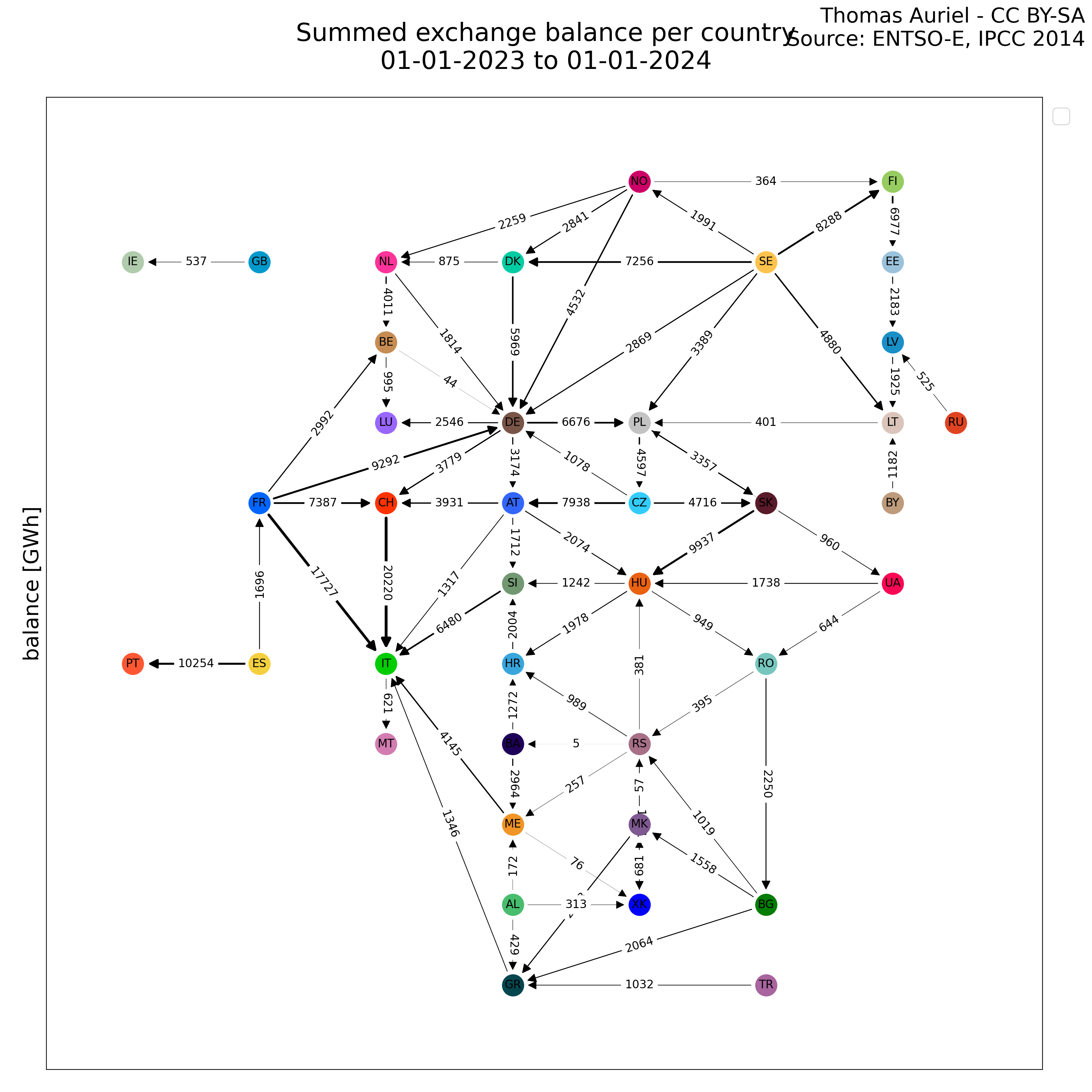
Graph representation
Graph network representations visualize complex interactions and electricity exchange among countries. Nodes represent individual countries, labeled with their iso code. Links illustrate the flow, direction, and intensity of exchanges, with wider links denoting greater exchange values. This representation aids in identifying countries with significant interactions and offers insights into international relationships.
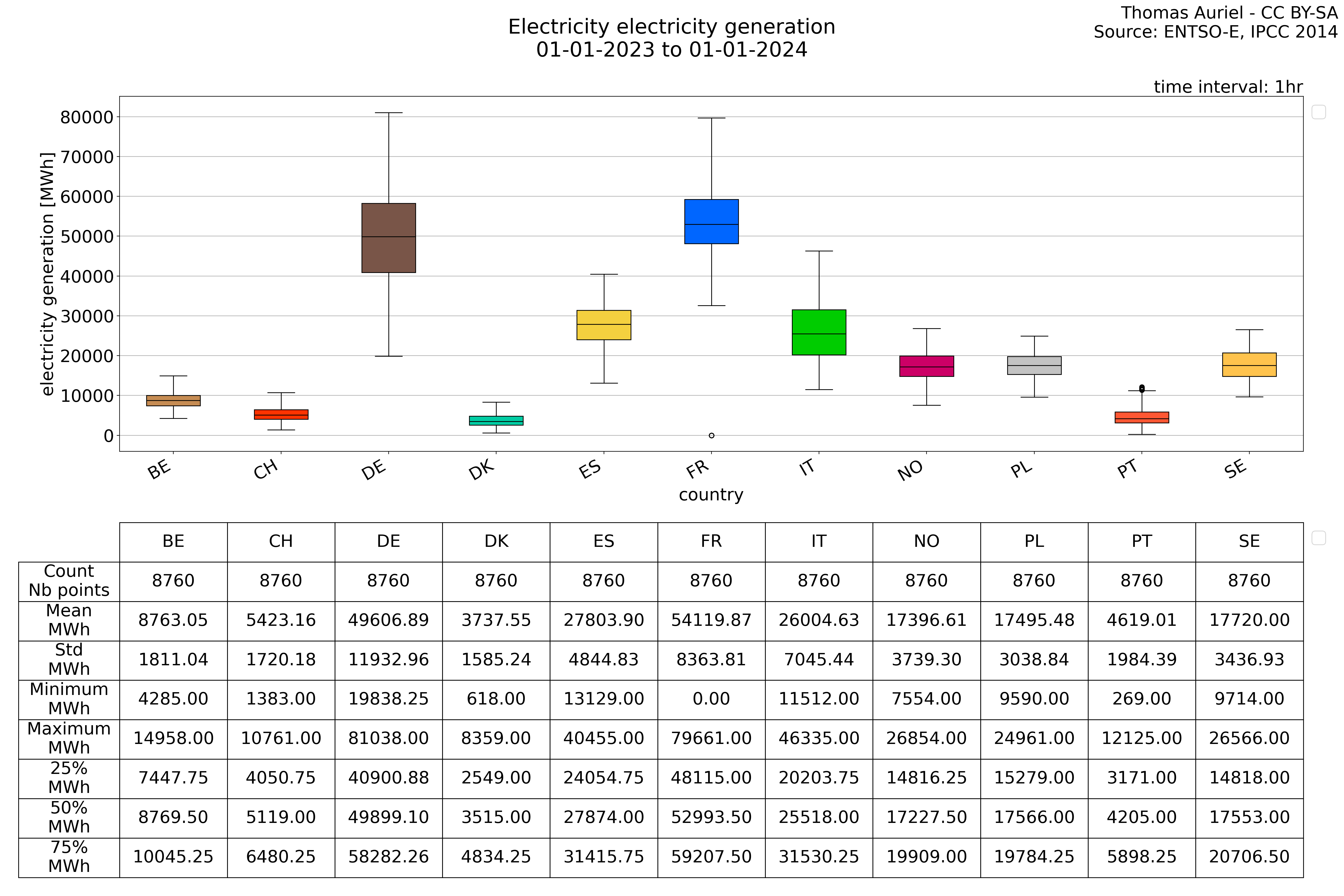
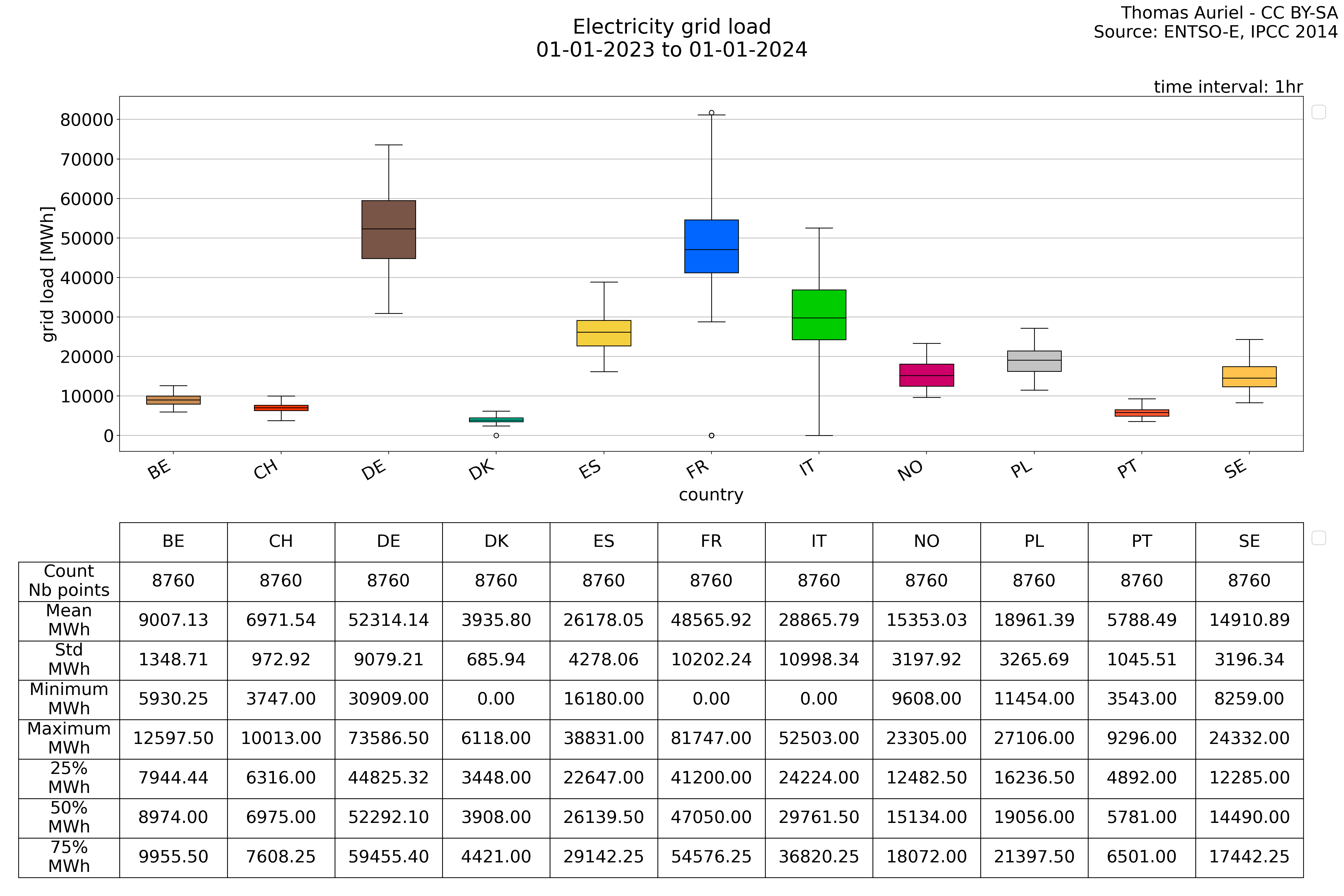
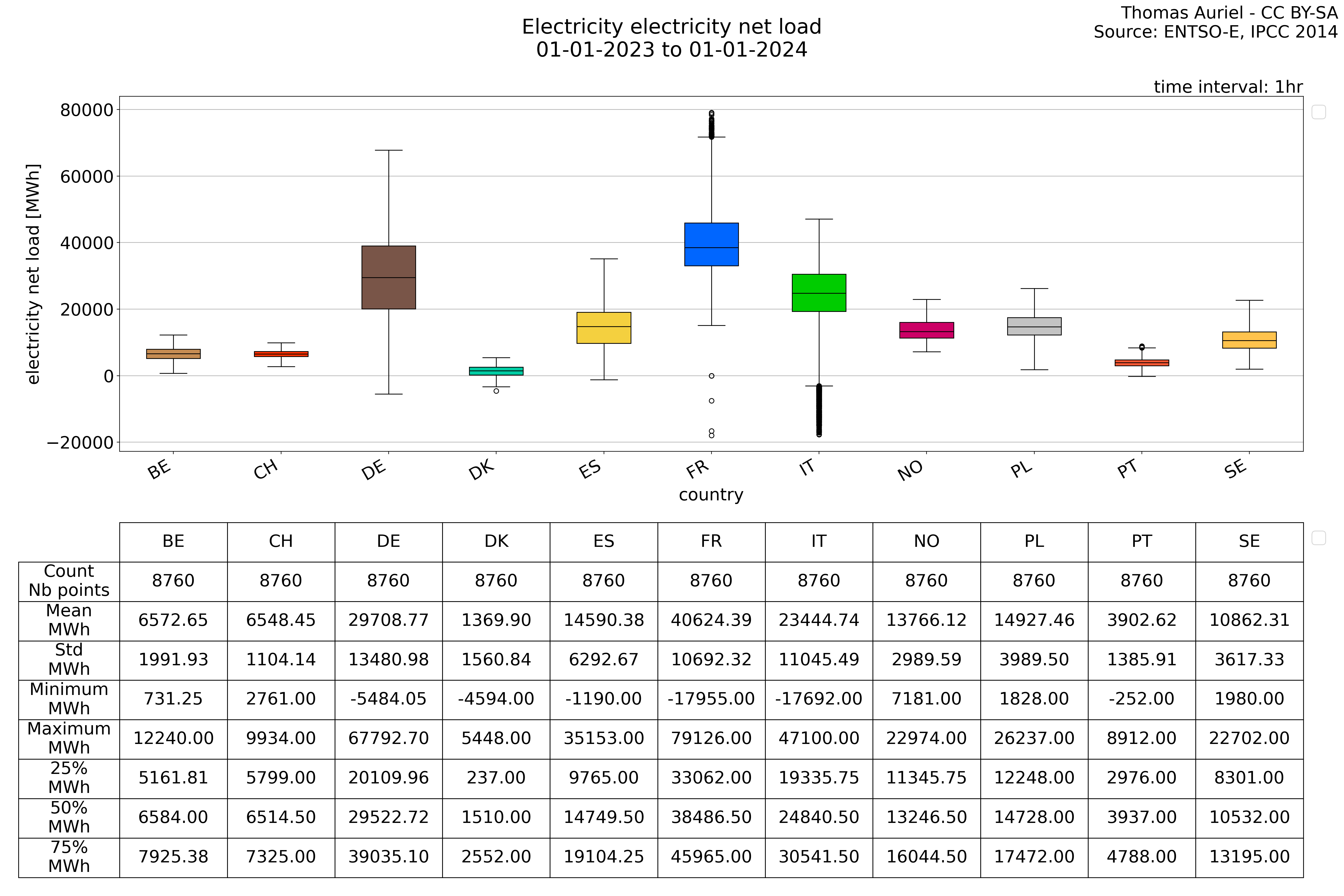
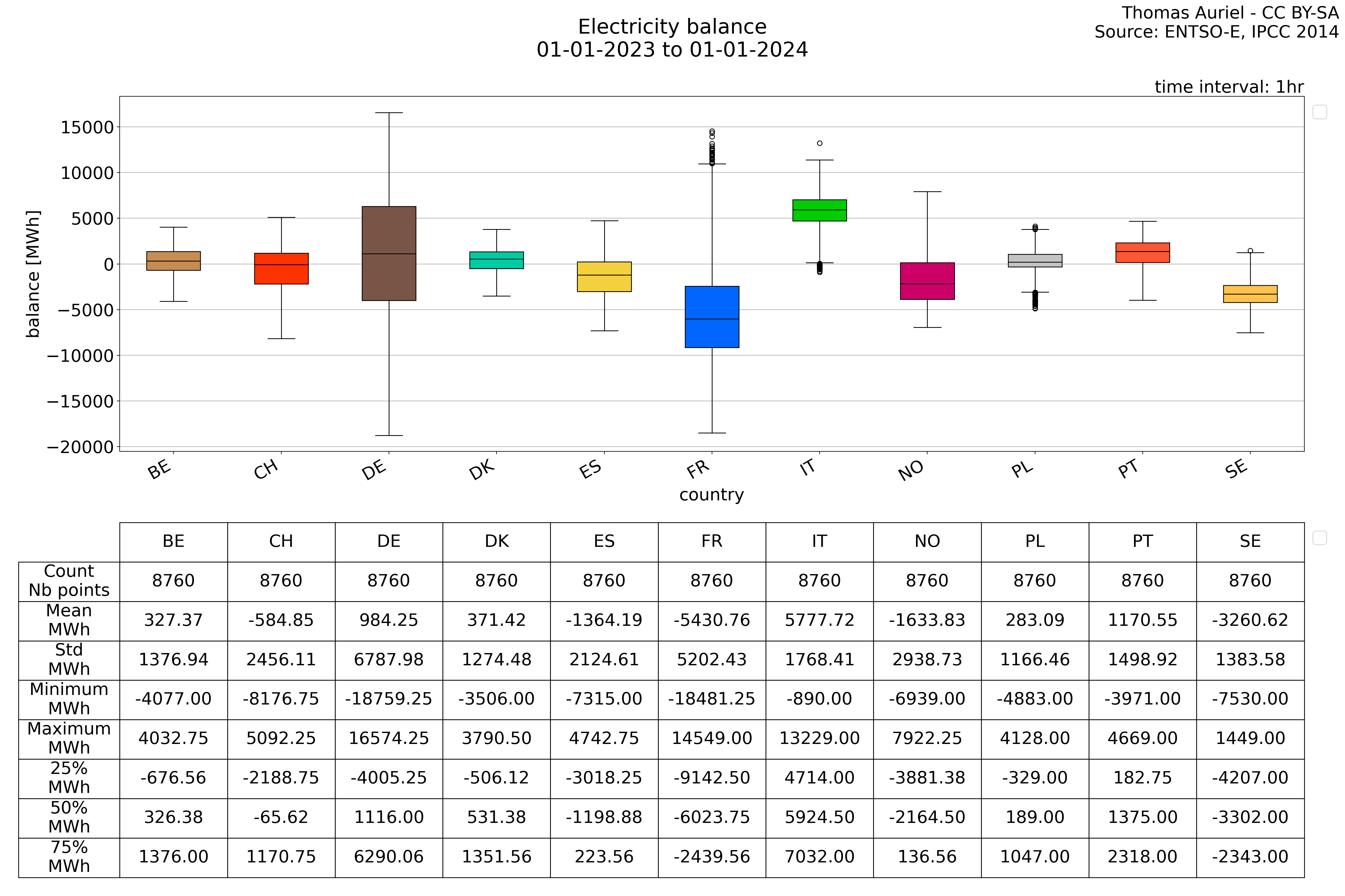
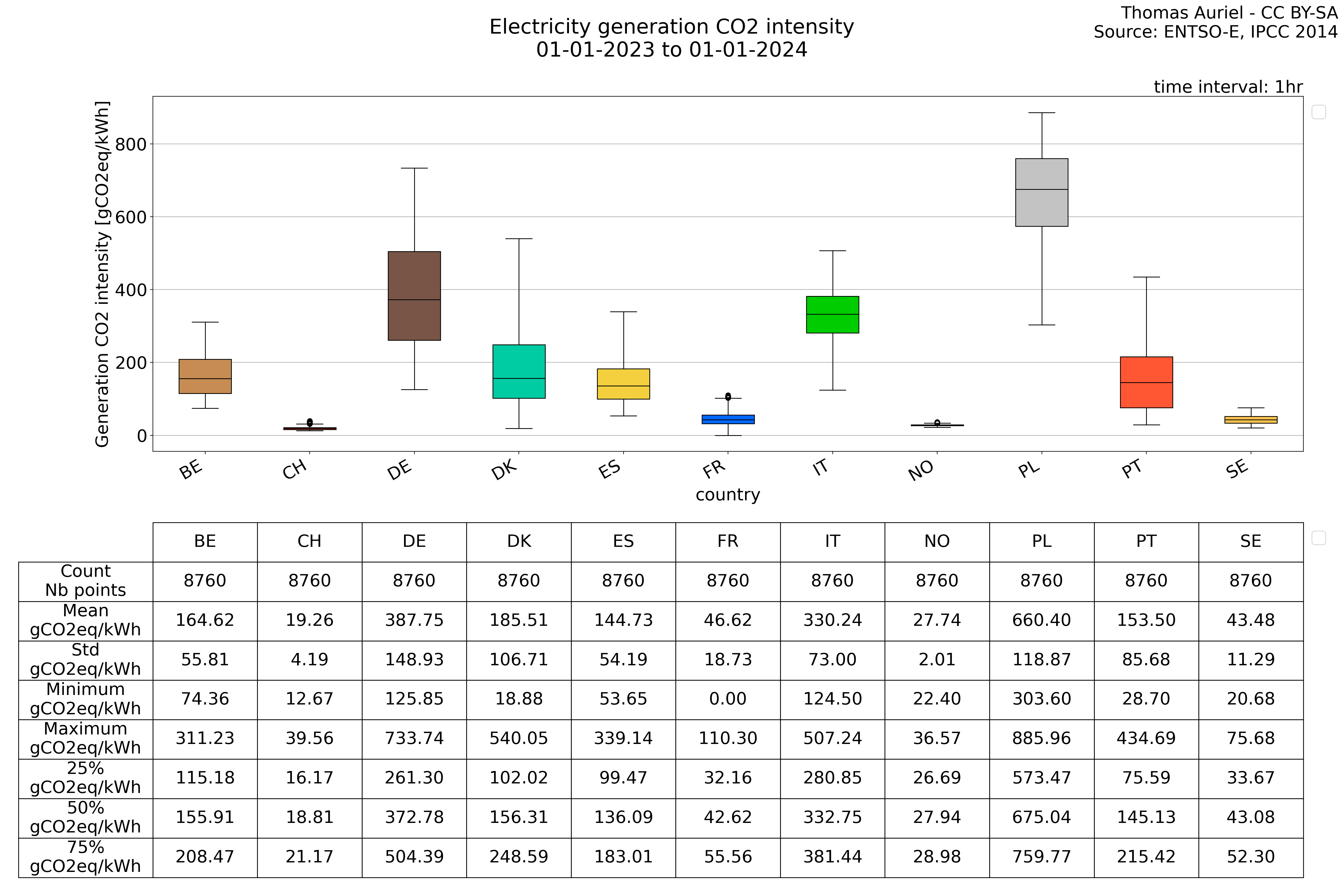
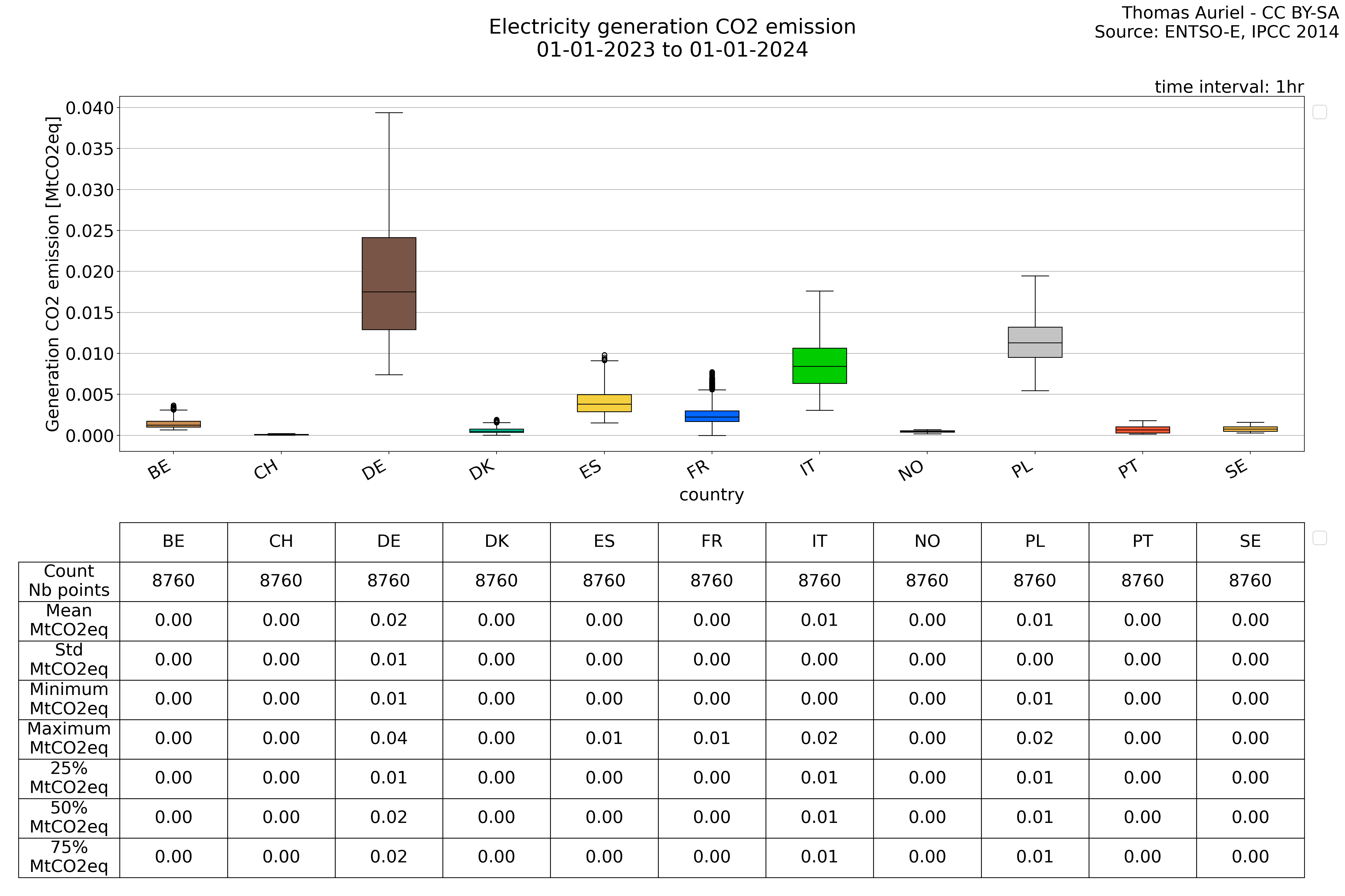
Box chart representation
A Box chart serves as a valuable tool to comprehend the distribution of data, whether categorized or organized by years. Here's a succinct explanation of the components within a Box chart:
-
Lower Whisker: Extending from the bottom of the chart, the lower whisker represents the range from the minimum data point to the 25th percentile, encapsulating the lowest 25% of the dataset.
-
Lower Box: Positioned immediately above the lower whisker, this box covers the range from the 25th percentile to the median (50th percentile), encompassing the interquartile range of the middle 25% of the data.
-
Upper Box: Located above the lower box, the upper box extends from the median (50th percentile) to the 75th percentile, representing the interquartile range of the upper 25% of the dataset.
-
Upper Whisker: Extending from the top of the upper box to the highest data point within the upper 25% of the data, the upper whisker signifies the range from the 75th percentile to the maximum data point.
Additionally, outliers are depicted as individual data points that lie significantly beyond the whiskers. Specifically, an outlier is identified as a data point whose deviation from the median is greater than two times the standard deviation. These outliers, characterized by their substantial deviation from the norm, are marked for further attention due to their distinctiveness.
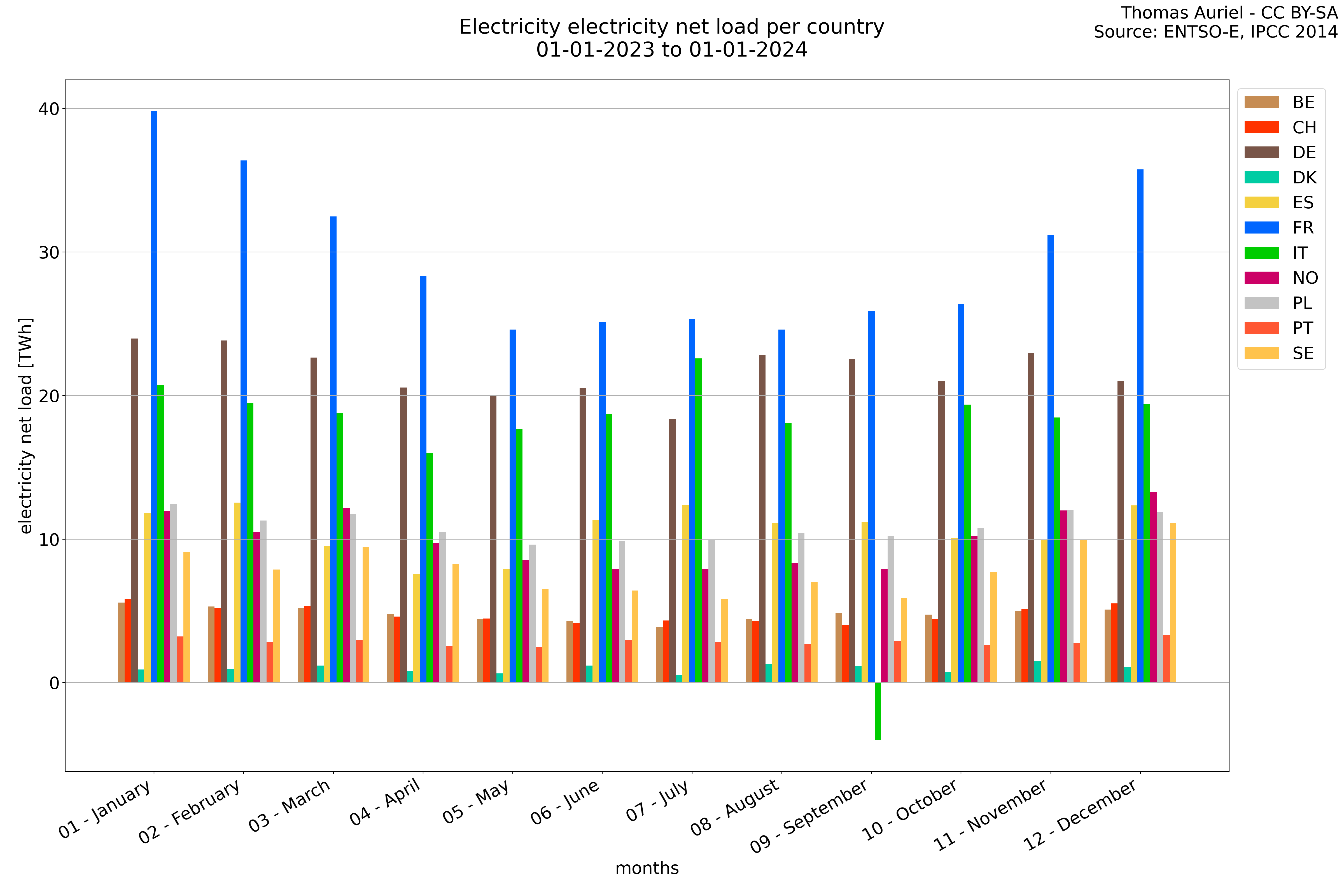
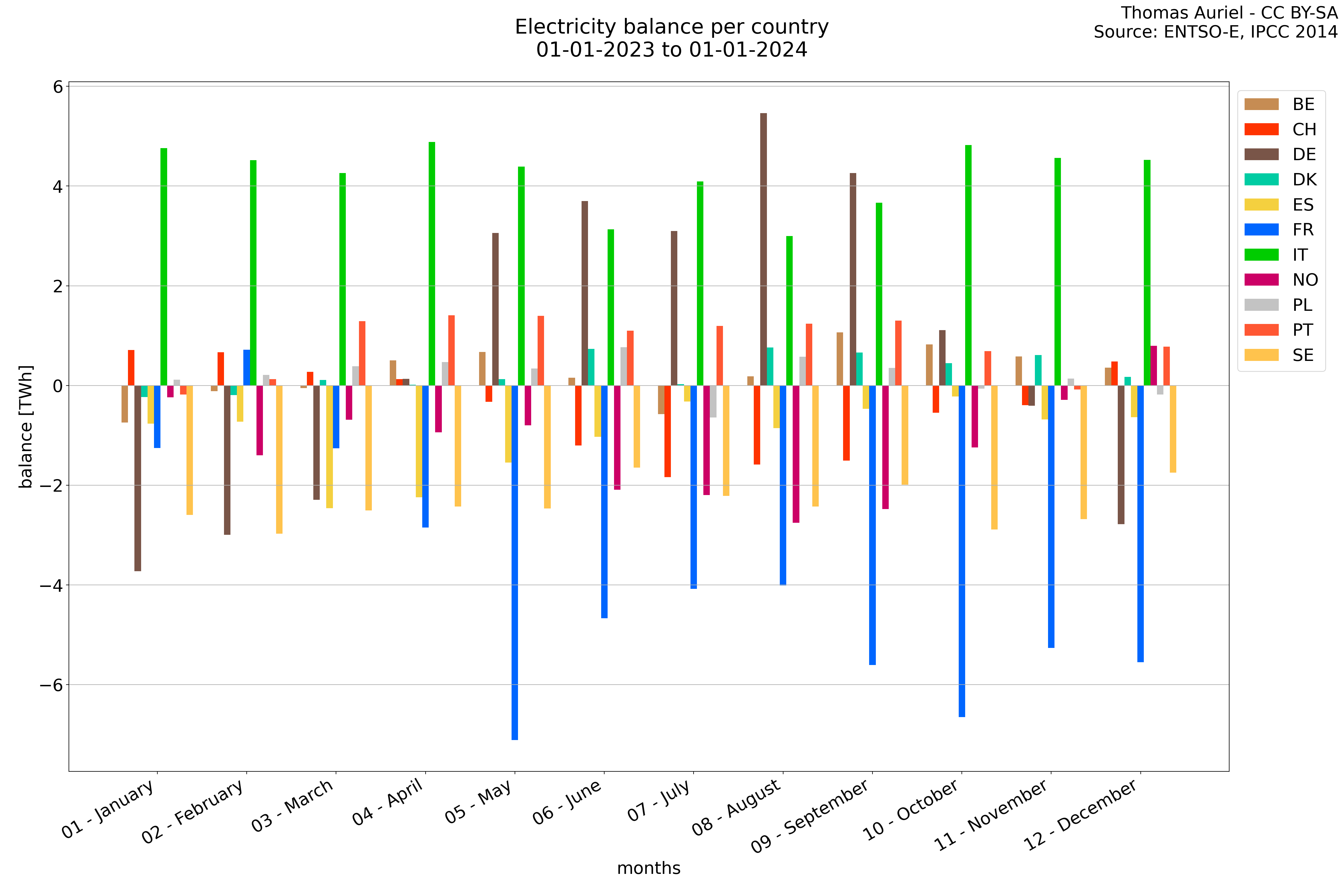
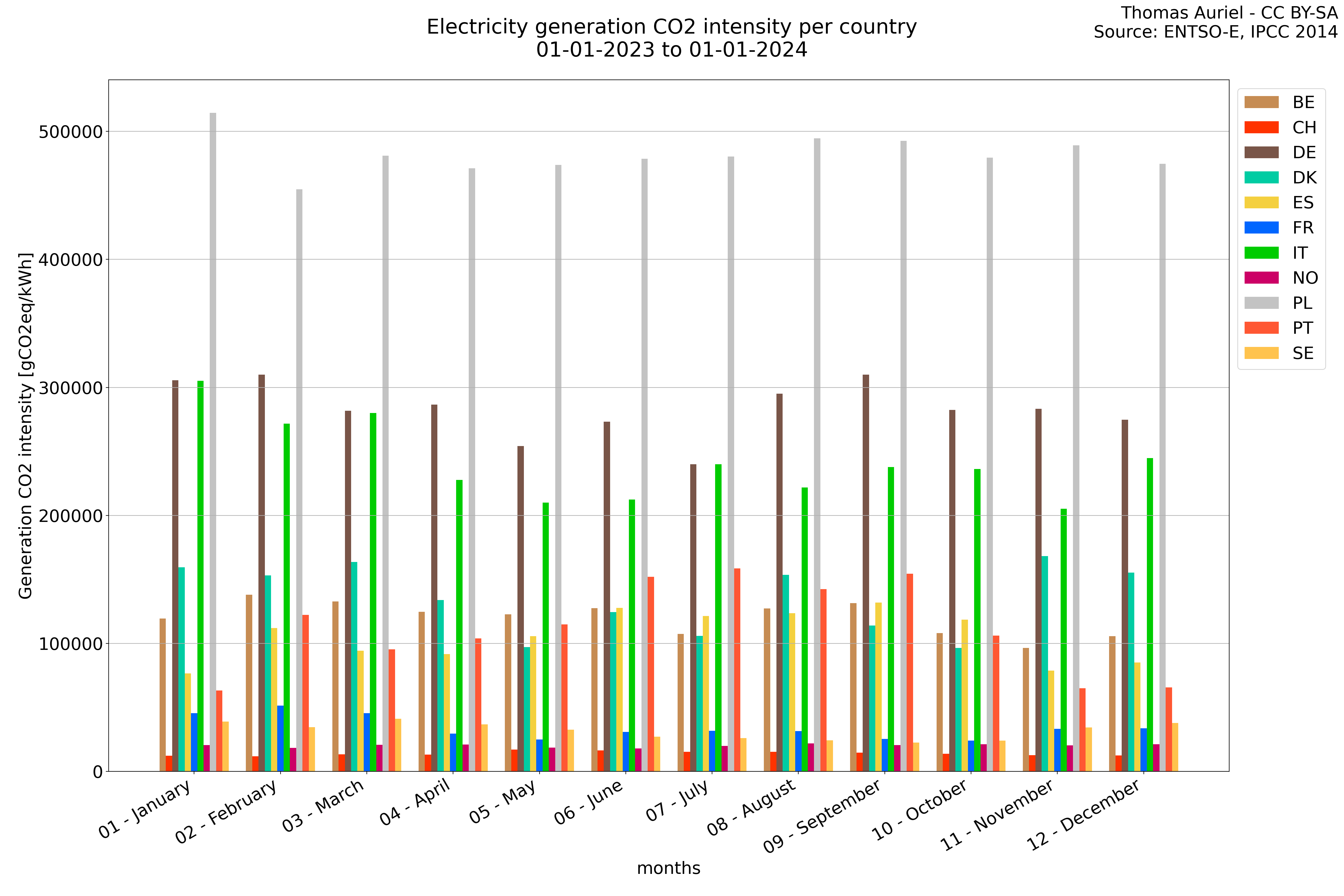
Periode representation
A periode plot takes a general view of the data by summing all the values over each month and presents them as a stacked bar plot. This visualization method allows for a clear understanding of how each country grid change over months. Then the Periode plot does not provide time-based trends but instead give an insight on the composition of the data within the chosen period.

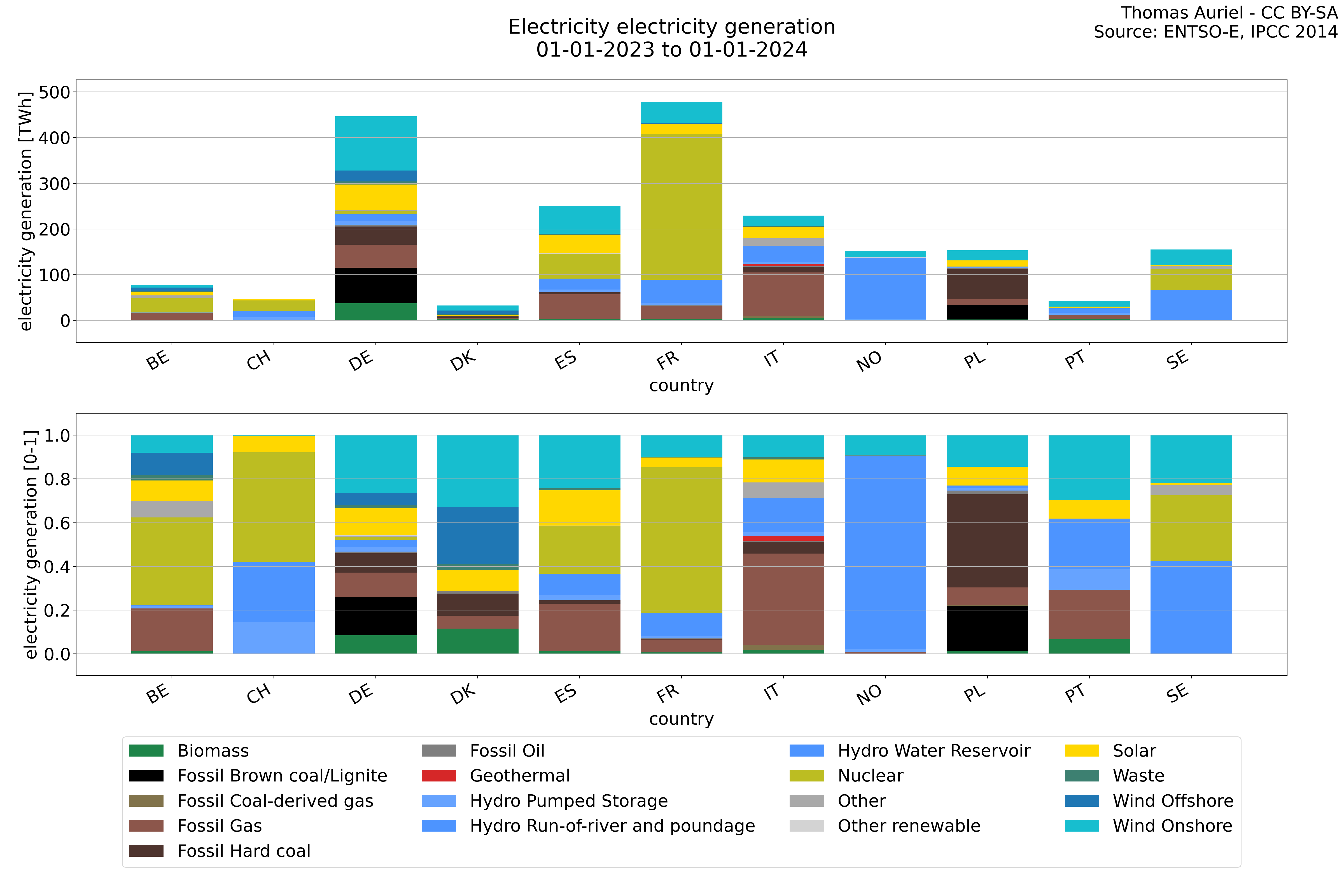
Bar plot representation
In these stacked bar plots, each bar represents a specific country. The bars are divided into sections that depict the decomposition of production, exchange, and CO2 emissions over the year. Two versions are presented: one displaying absolute values, and the other showing relative values. In the absolute values plot, each country's bar illustrates the absolute amounts of these components during the year. The relative values plot showcases the proportion of each component within a country's data for the entire year. These stacked bar plots offer insights into how production, exchange, and CO2 emissions vary across countries, aiding in comparative analysis.


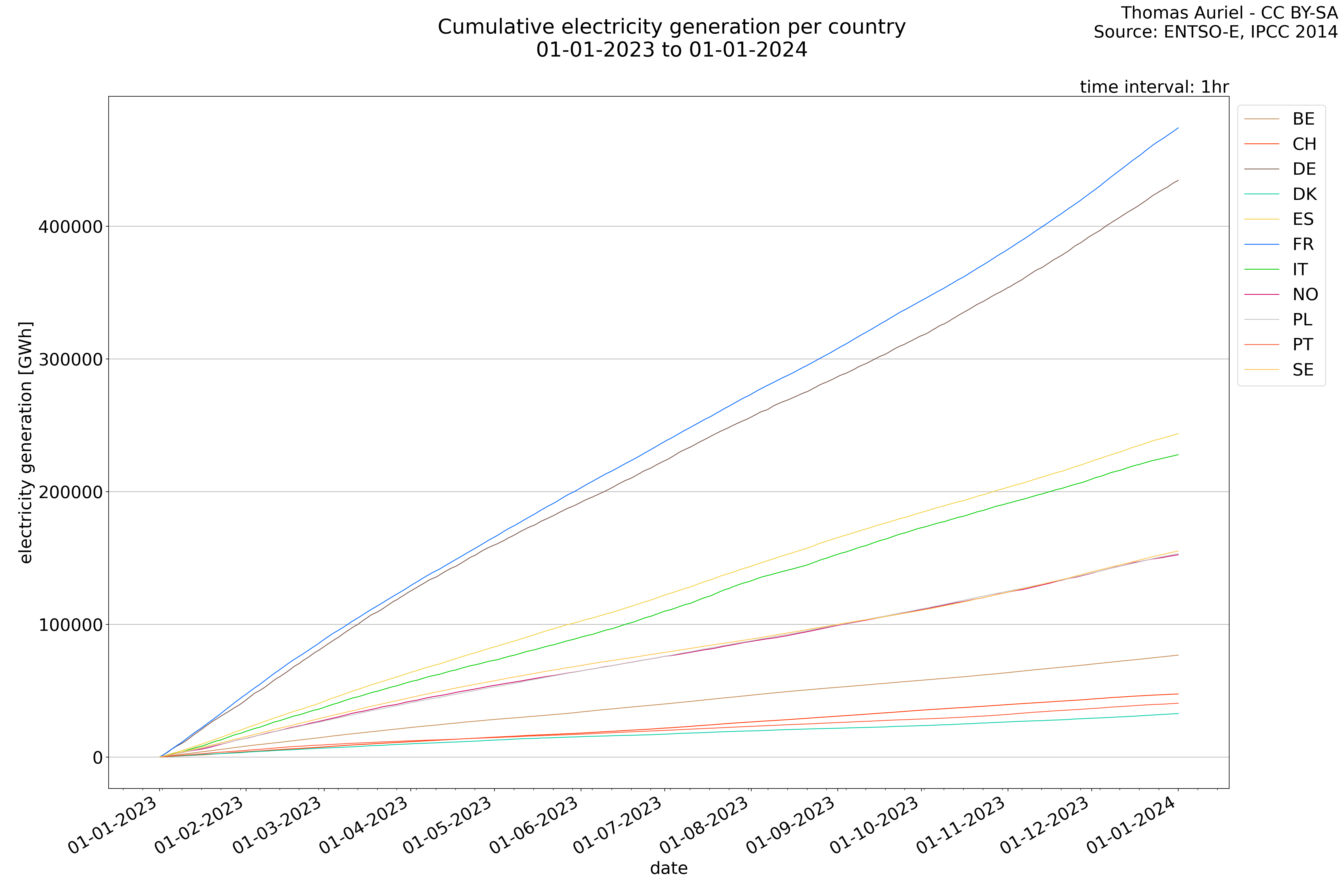
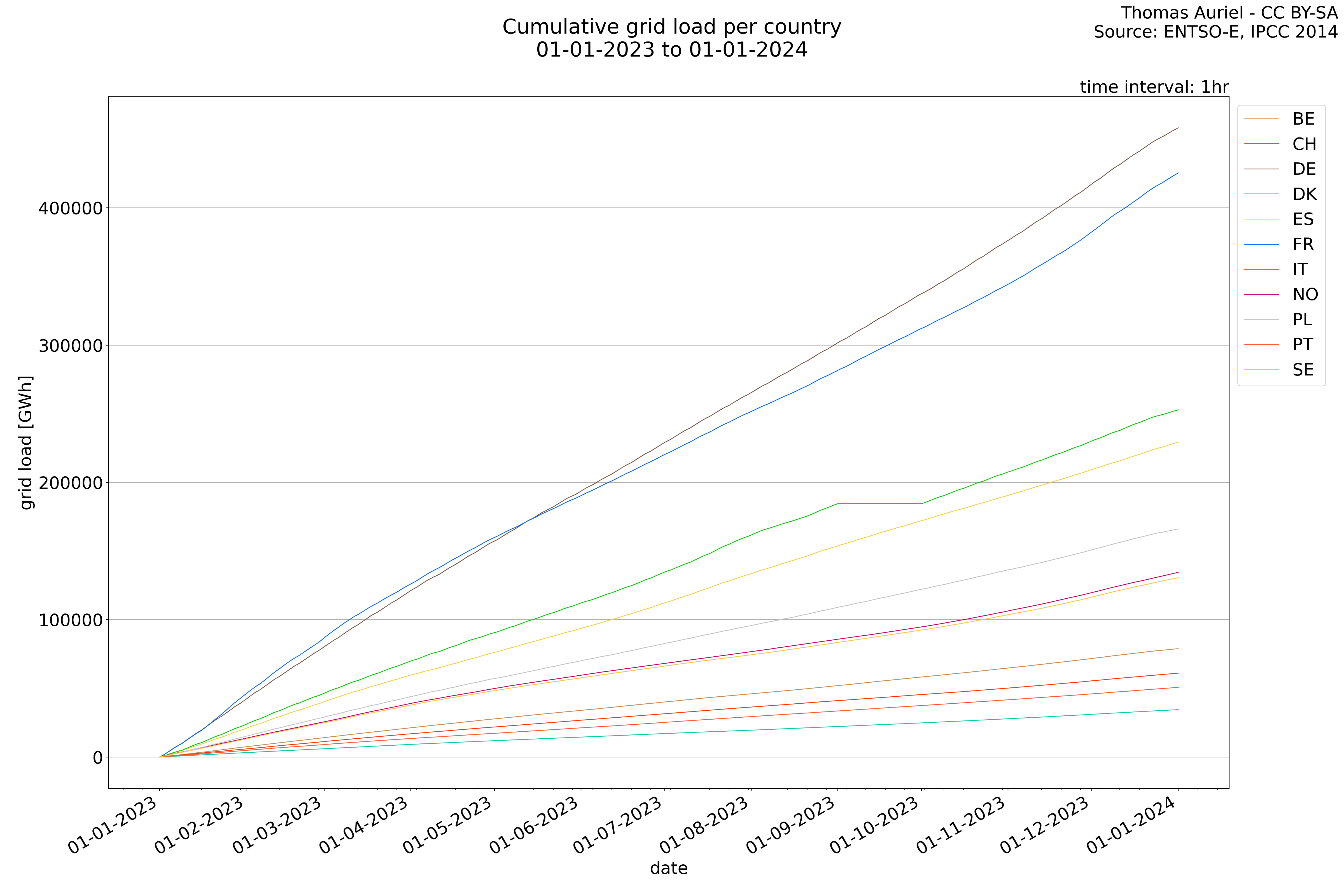
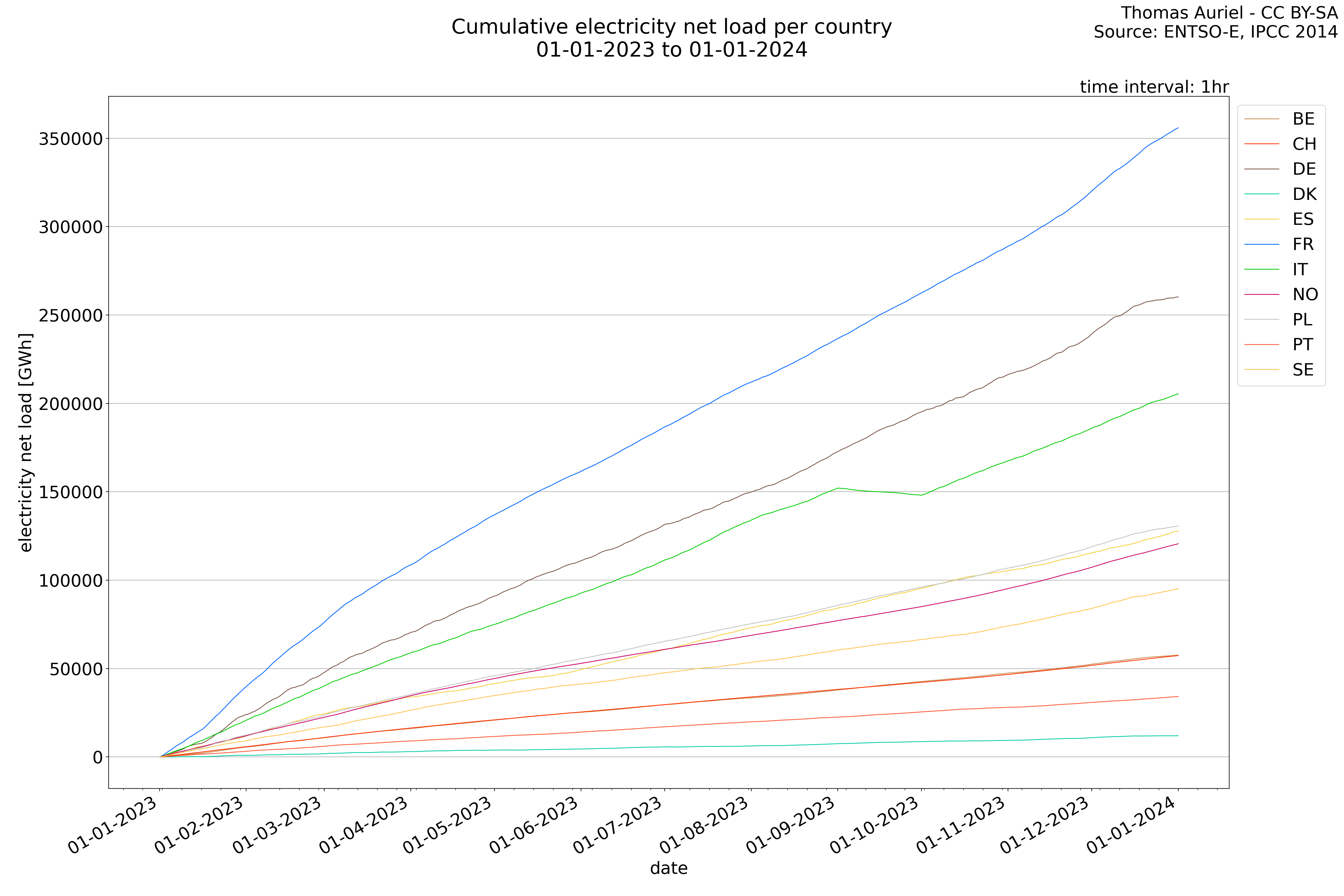
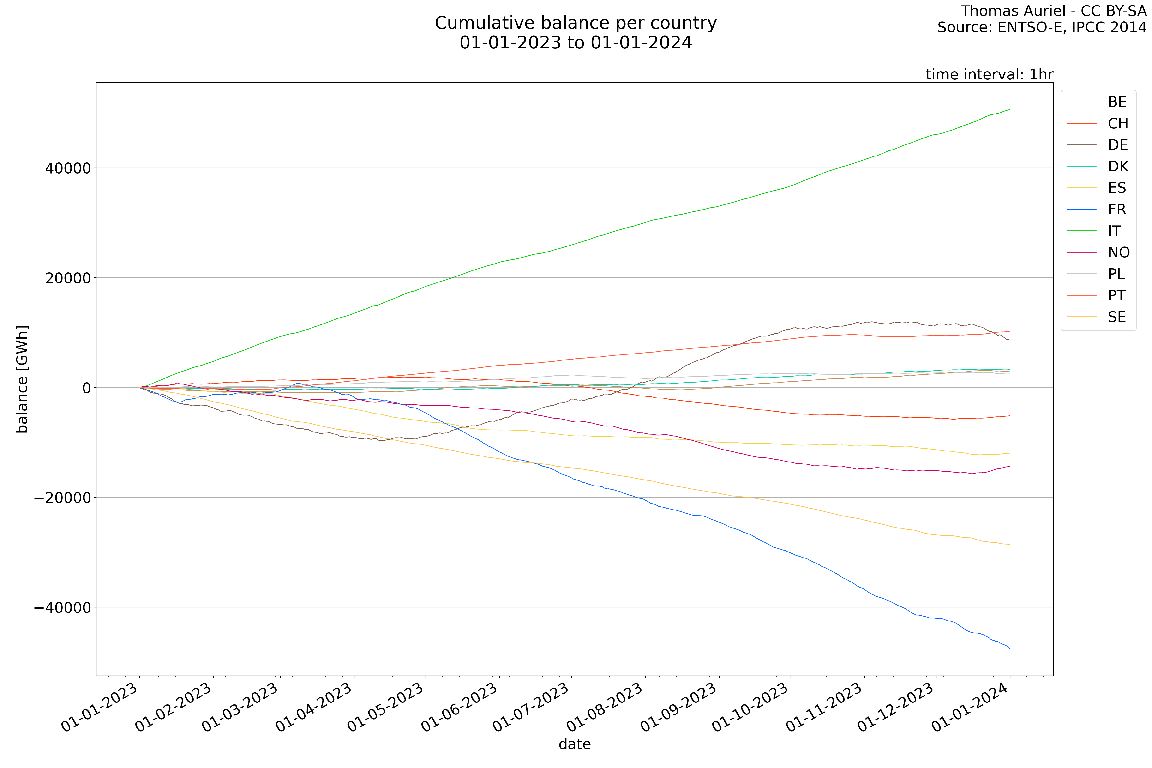
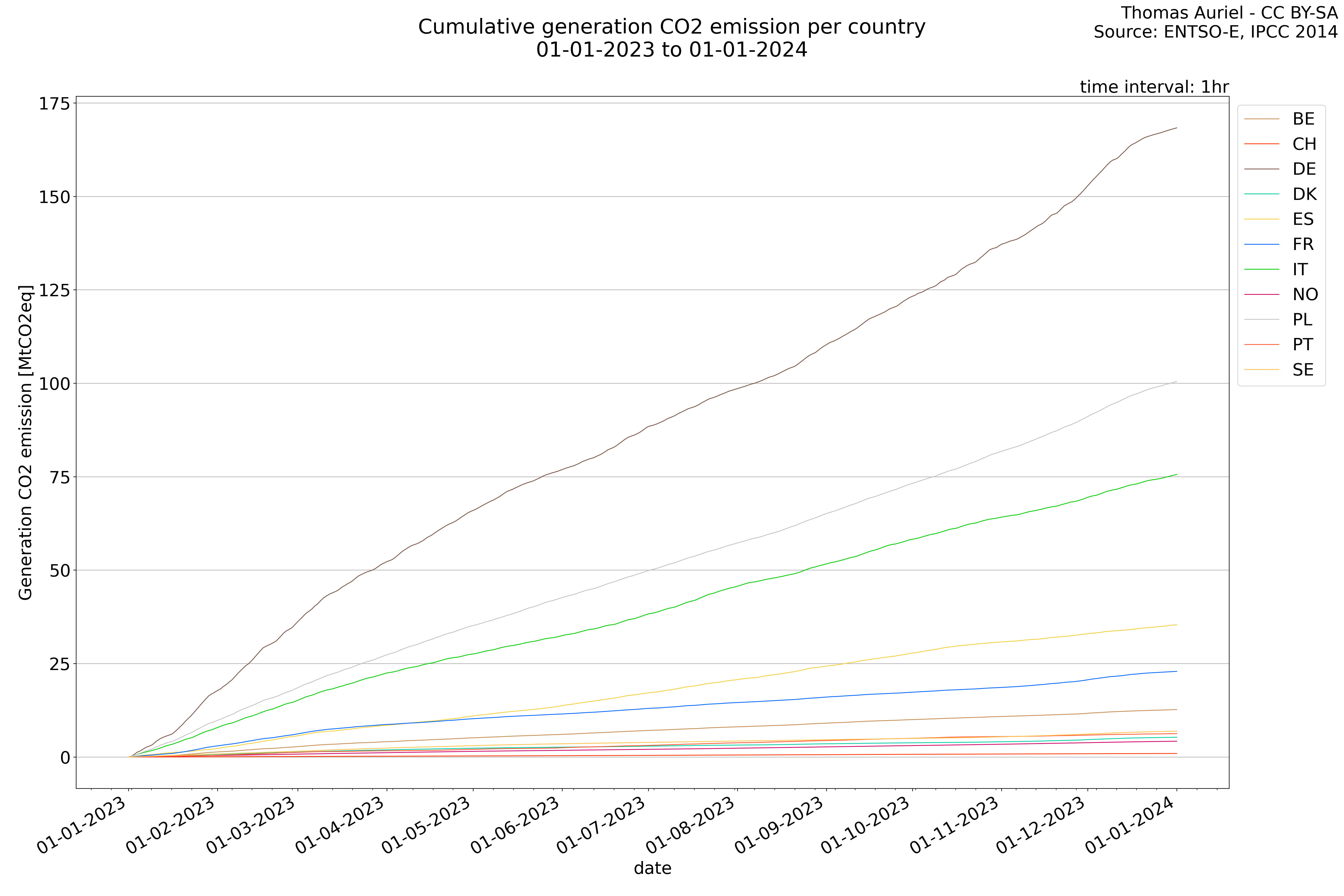
Cumulative representation
In these cumulative line plots, the x-axis spans the entire year, with hours as individual data points. The y-axis represents the cumulative total of production, exchange, consumption, and data emissions. Each line on the plot corresponds to a distinct country, providing a comprehensive view of how these variables evolve throughout the year. These plots offer insights into the annual evolution for each country.
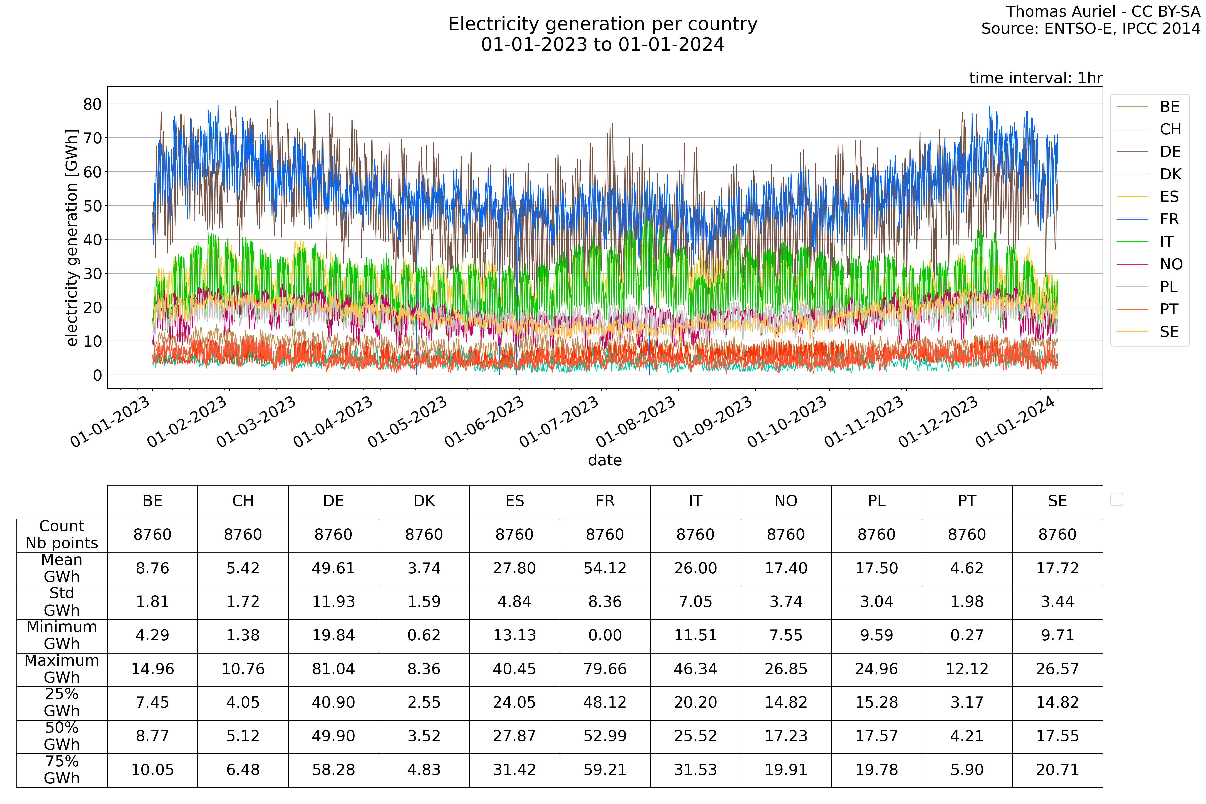
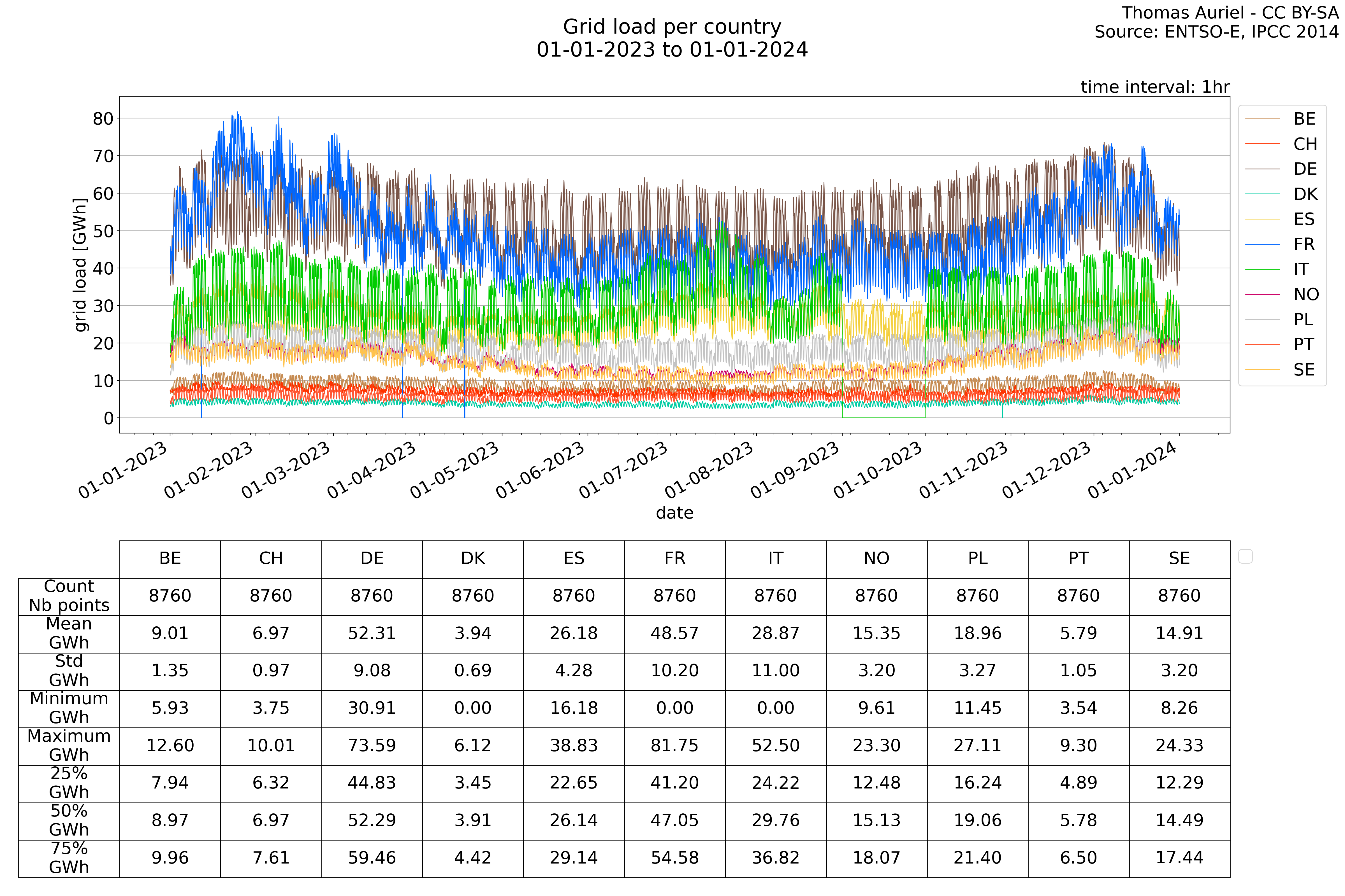
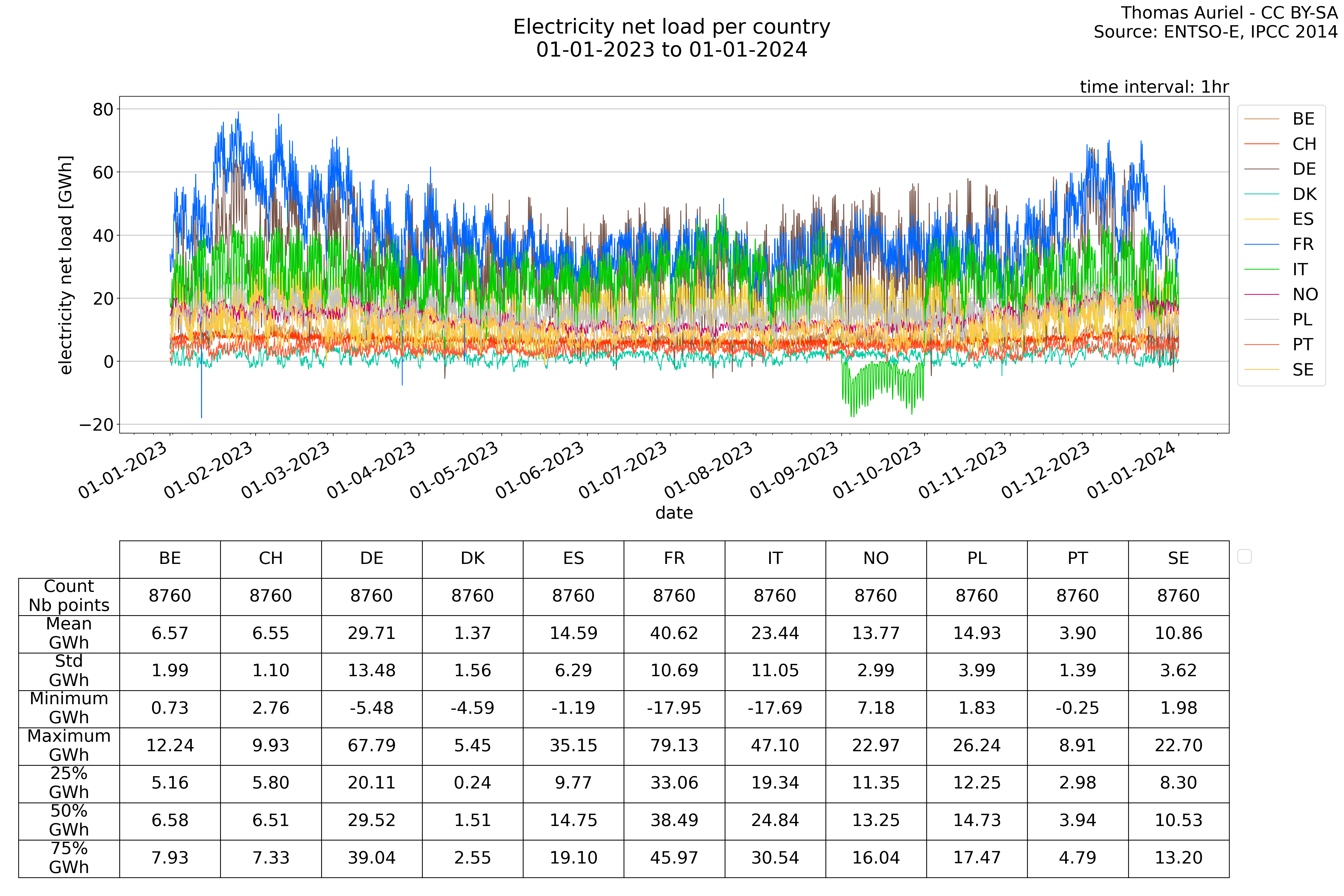
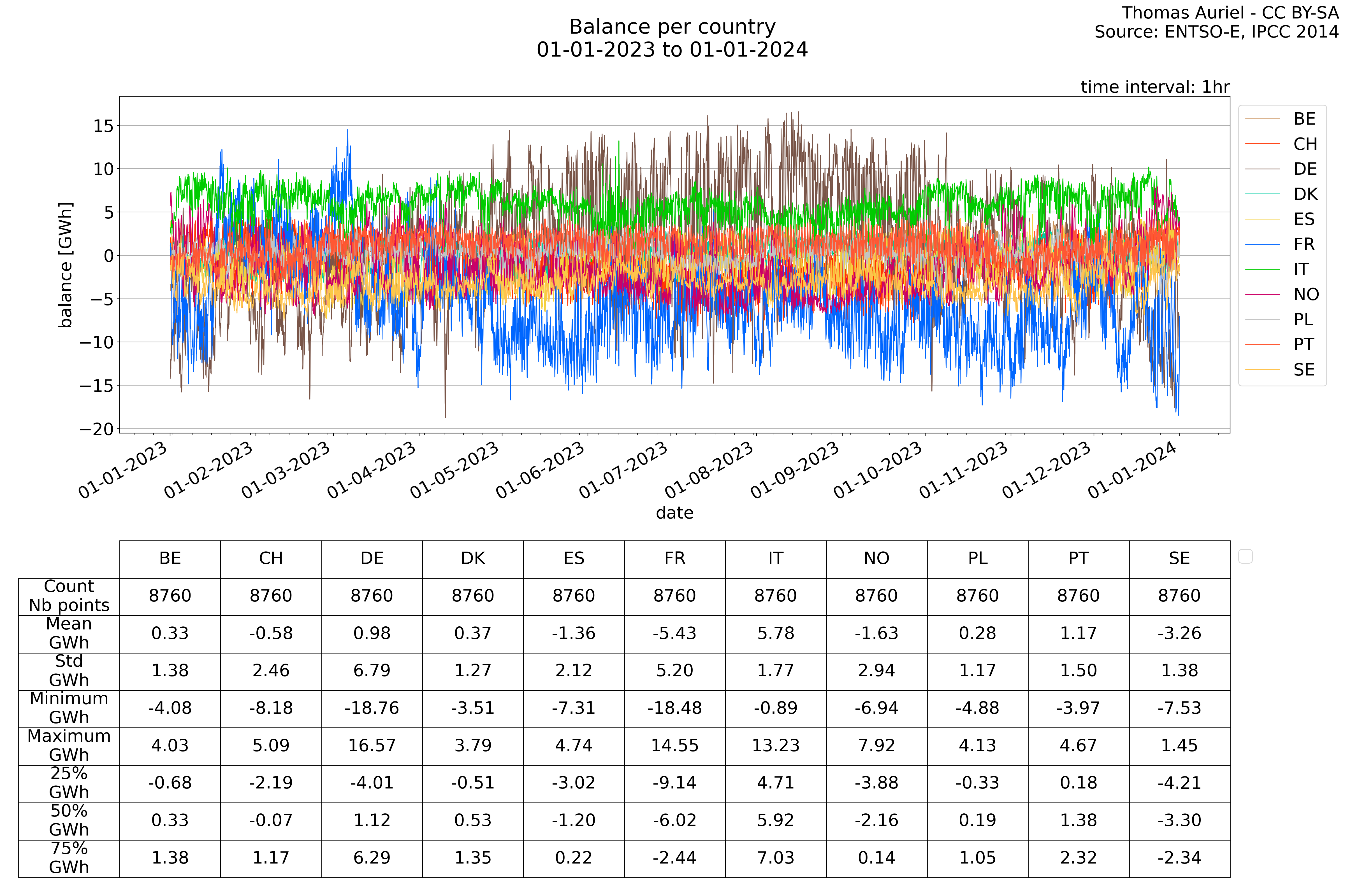
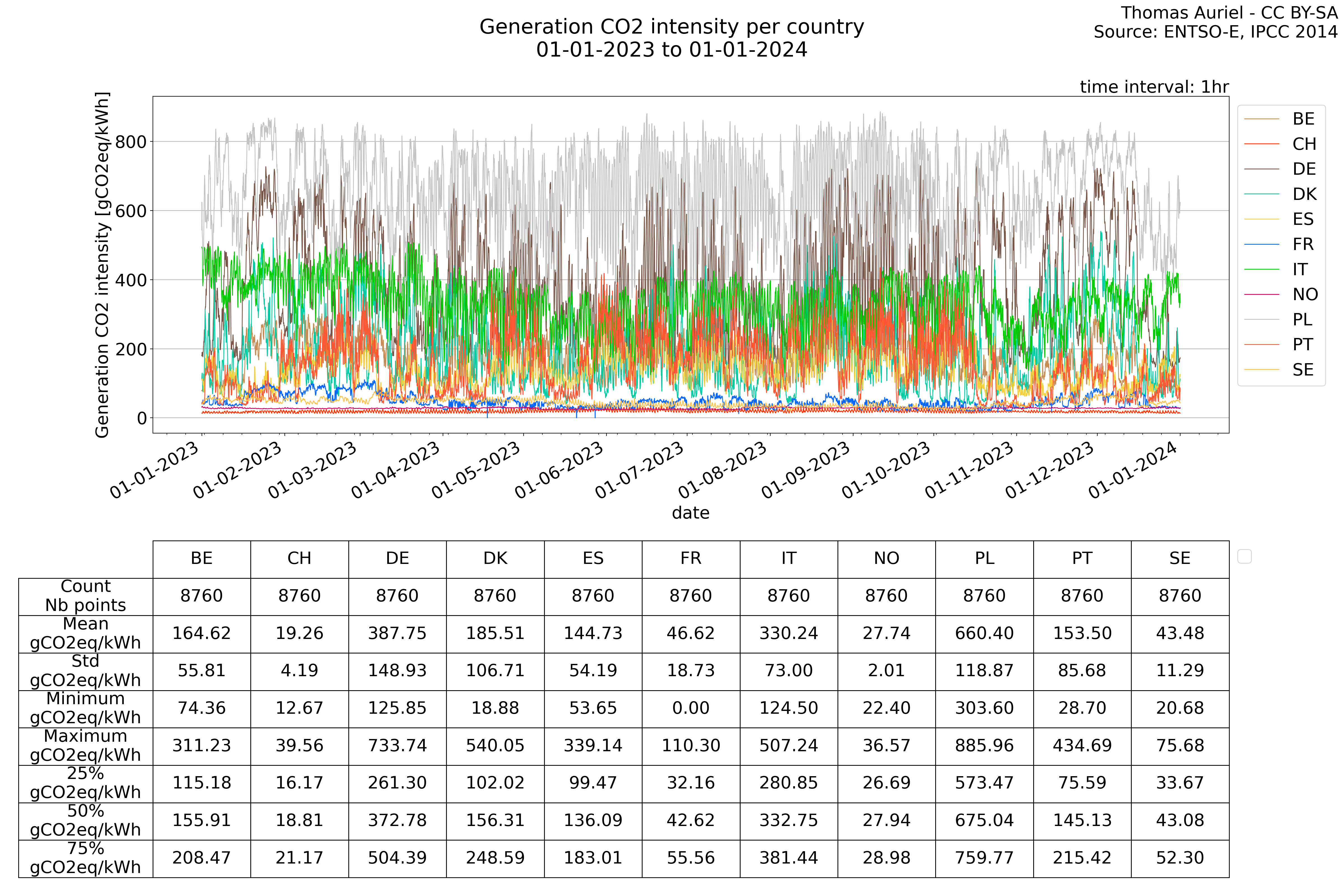
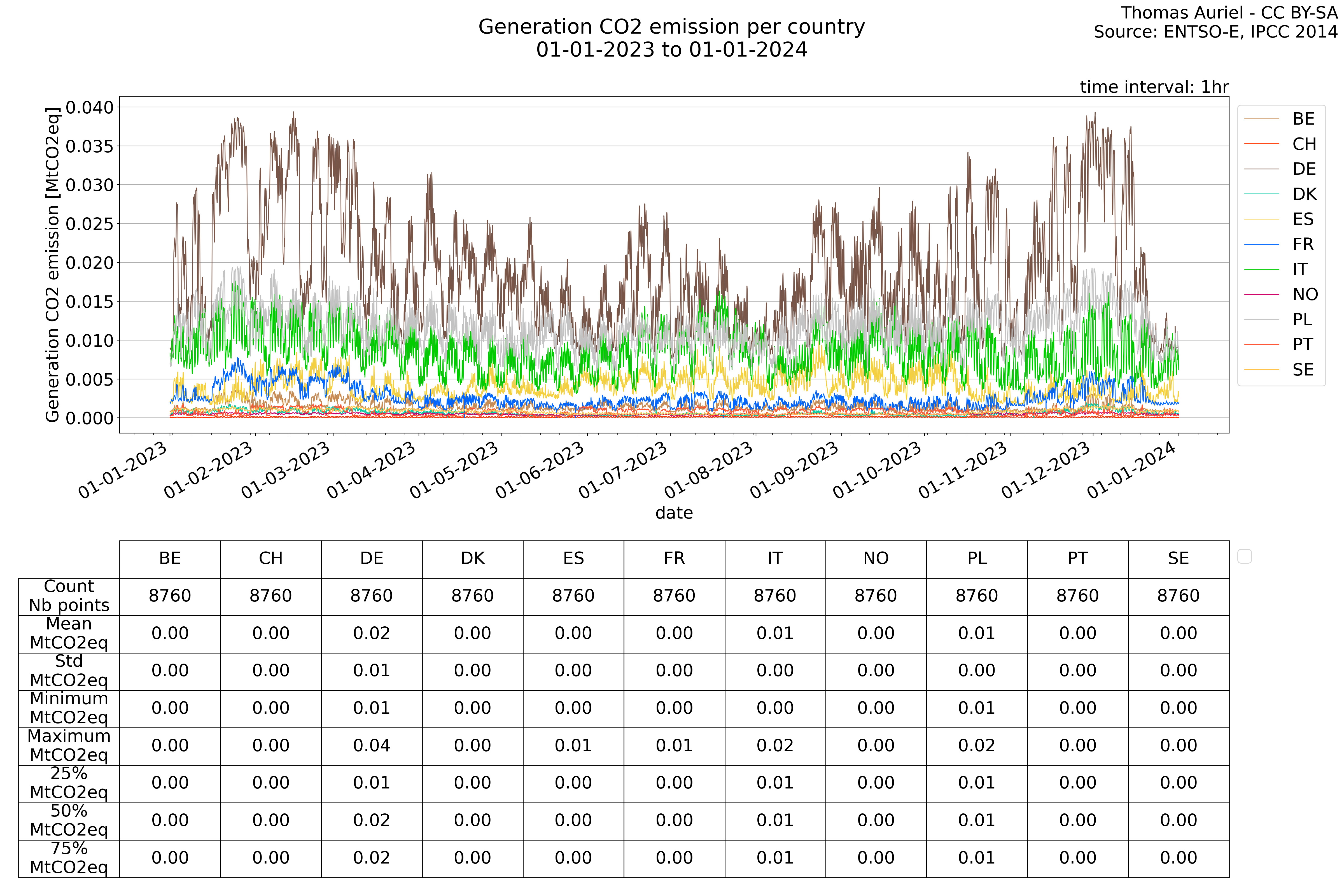
Linear representation
In these hourly line plots, the x-axis spans the entire year, with hours as individual data points. The y-axis represents the values of production, exchange, consumption, and data emissions, but unlike cumulative plots, these plots are designed for quality control purposes. Each line on the plot corresponds to a specific country and is used to identify data irregularities, holes, or artifacts that may occur within the year. By examining these plots, it is possible to spot discrepancies or missing data points in the hourly records, ensuring data integrity.