Estimation of the consumption in an electrical grid using Markov and Leontief approaches
Thomas Auriel, 20th December 2023
In this article I present to you a way to estimate how production and consumption propagate into a grid.
Introduction
There has always been a difficulty in defining what is really consumed on a network for one particular actor. Considering only the production, it is complex to estimate what is really consumed by users. Production changes over time, interconnections and storage helps to match the load at any time. And since all the consumers are connected to all the producers it is not trivial to attribute part of a production to a consumer.
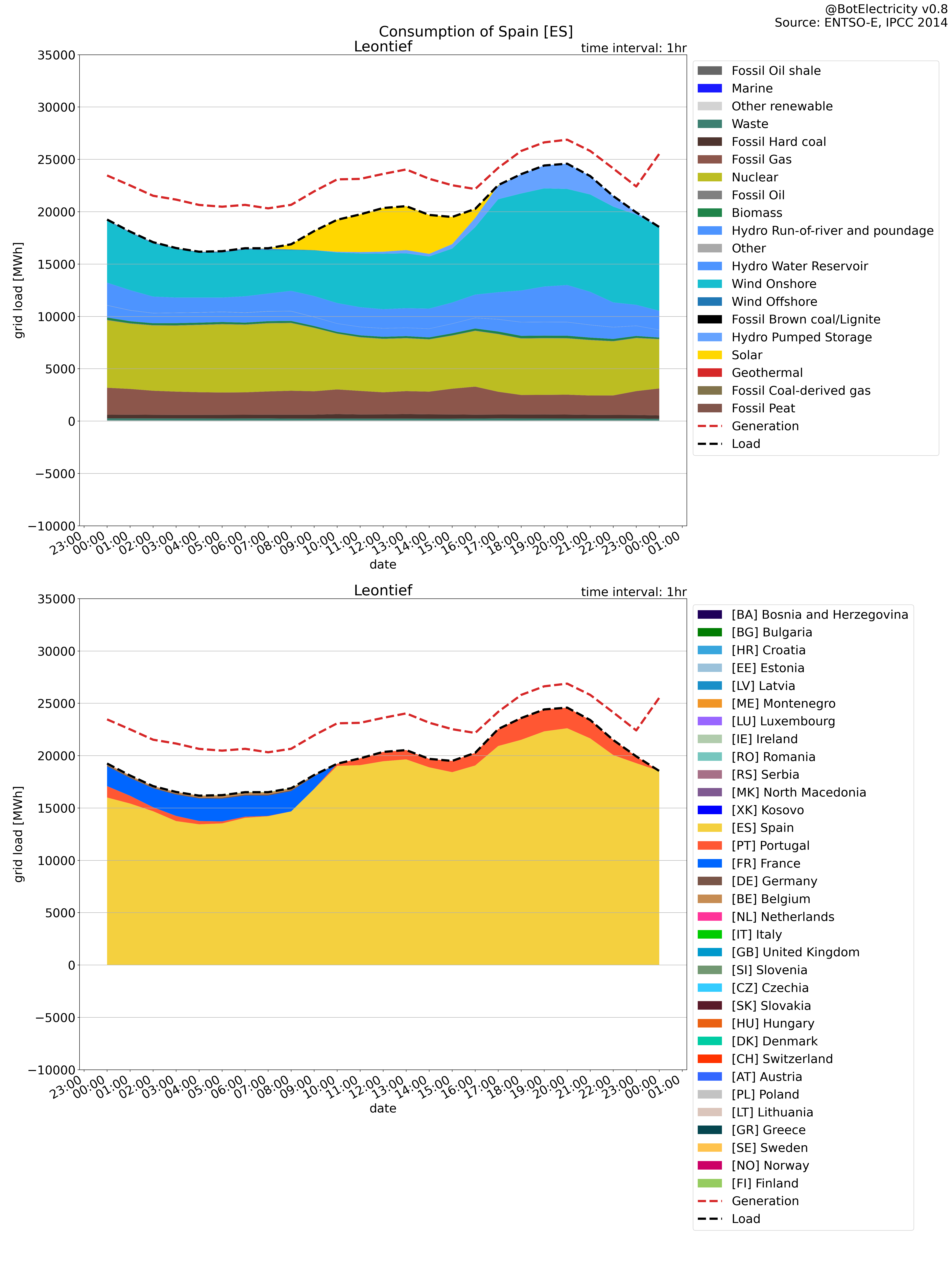
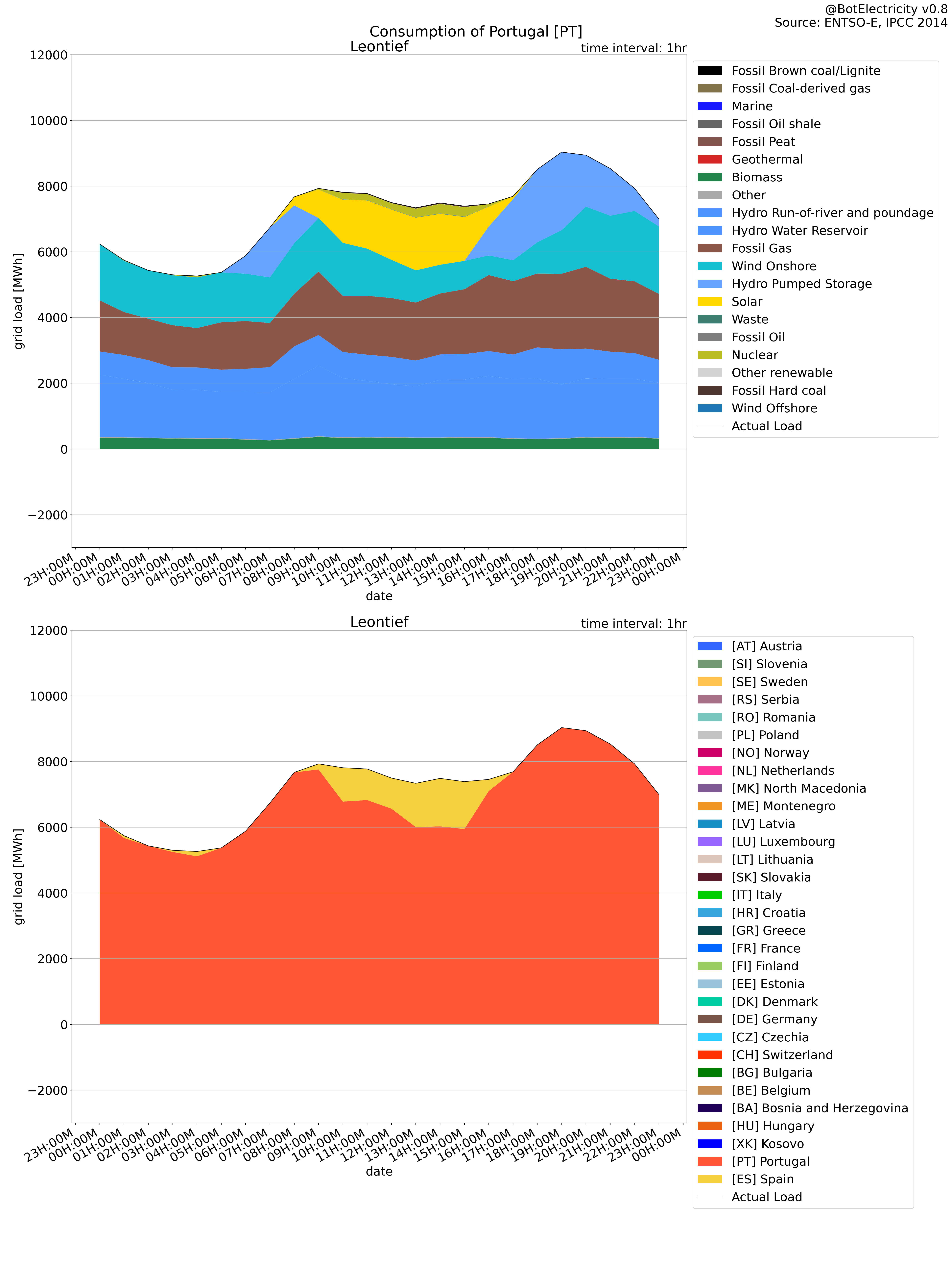
In the next figures, you can see a difference between the production and the consumption in Spain and Portugal. The production is higher than the consumption.
The colors represent the production. And the line represents the consumption. The balance and storage are added to see their impact. Positive balance/storage means they behave like production. Negative balance/storage means they behave like consumption.
Attribution strategy
To associate production to consumption, several strategies are possible. We can cite at least:
- Average production match the average consumption (over a period of time, attribute to each consumer the average production according to the volume they consumed);
- Marginal production attribute to marginal consumption (when a consumer increase the load, we attribute the last production method called on the grid);
- Guaranty of origin (a consumer pays directly for the production for the electricity consumed and the attribution is done no matter the physical state of the grid);
- etc.
These methods allow us to attribute consumption. But it is always required to accept assumptions (and their consequences). Discussions can emerge on this and depending on the view on the electrical grid a method will be considerate valid compare to others.
It is possible to have an approach using mathematical definition. I propose with this tool to consider the electrical grid as a Markov chain or a Leontief approach.
The Markov approach shows where the production end.

The Leontief approach shows where the load is drawing its energy.
Both approaches should give the same numbers. However, we are dependent of the quality of the data. Production, load and balance never match perfectly. The previous examples show this. It means the electricity flow in the grid is not perfectly captured and the data will always show a difference. The true values should be between the two results provided by the two methods.
Explanation
To perform the calculation, we consider the European grid as a graph. This graph allows us to simplify each element as a node. Then, each generation type, country, load and exchanges are similar to nodes. The directed edges are the exchange between them.
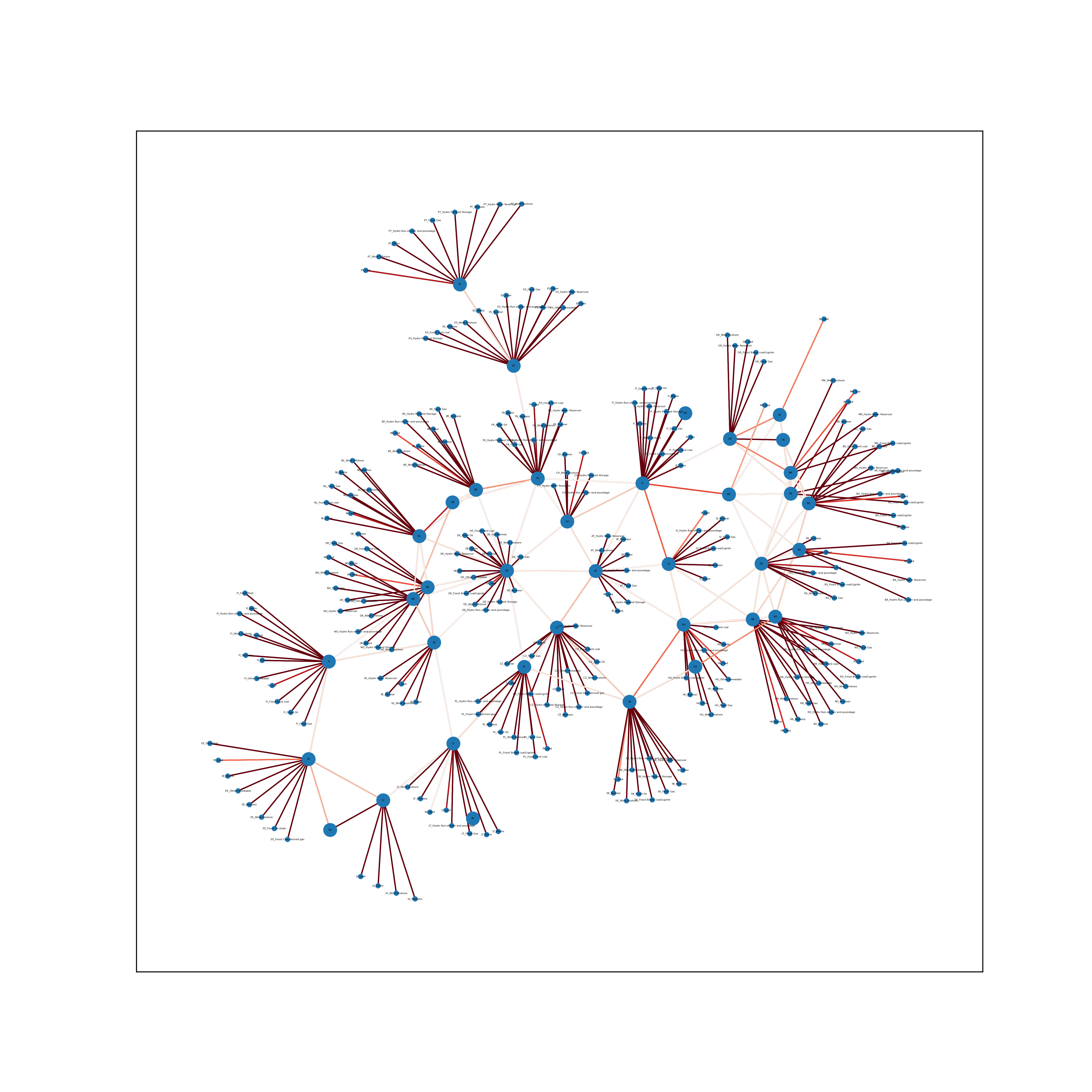
The graph is similar to a Markov chain.
When a MWh is at node, it is split between each edge leaving the node. The division is proportional to the weight of the edges. And because the grid does not melt down and work correctly, we know there is a solution where an equilibrium is found and all the generated power ends in a storage or in a load.

Markov approach: Where does end the production in the graph (what is available to consume)
It is interesting also to notice that it is possible to follow the load. This is similar to a Leontief approach.

Leontief approach: Where the consumption end (what is driving the production).
Assumptions
Like all other methods, assumptions must be considered to understand the validity of the data:
- Each country is considerate as a bidding zone. Some countries are divided into bidding zone. It is possible to use this level of detail to do the computation. This is not done in the current tool. This will affect the number of nodes and edges in the graph.
- In a country/bidding zone, electricity is supposed to be perfectly mixed and distributed.
- Each MWh has the same behaviour independently of its origin. Electrons are not distinguishable.
- A MWh can only transit from a country to another only if they are linked. It needs a physical link.
- Storage is considered as load or generation depending on their state. There is no negative MWh.
- Information of the source of the electricity is lost in storage. It's possible to know which source feeds a storage. It should be possible to know it later when the energy leaving a storage but this is not implemented yet.
Some mathematical assumptions need to be respected:
- If the grid is divided in two grids with no exchange between them, then the method cannot work. You have to apply the method to each graph separately.
- There must be no internal infinite loop. For instance, two countries exchanging energy together without consuming it (since it is not possible it is not an issue).
Example for a country with more exchanges
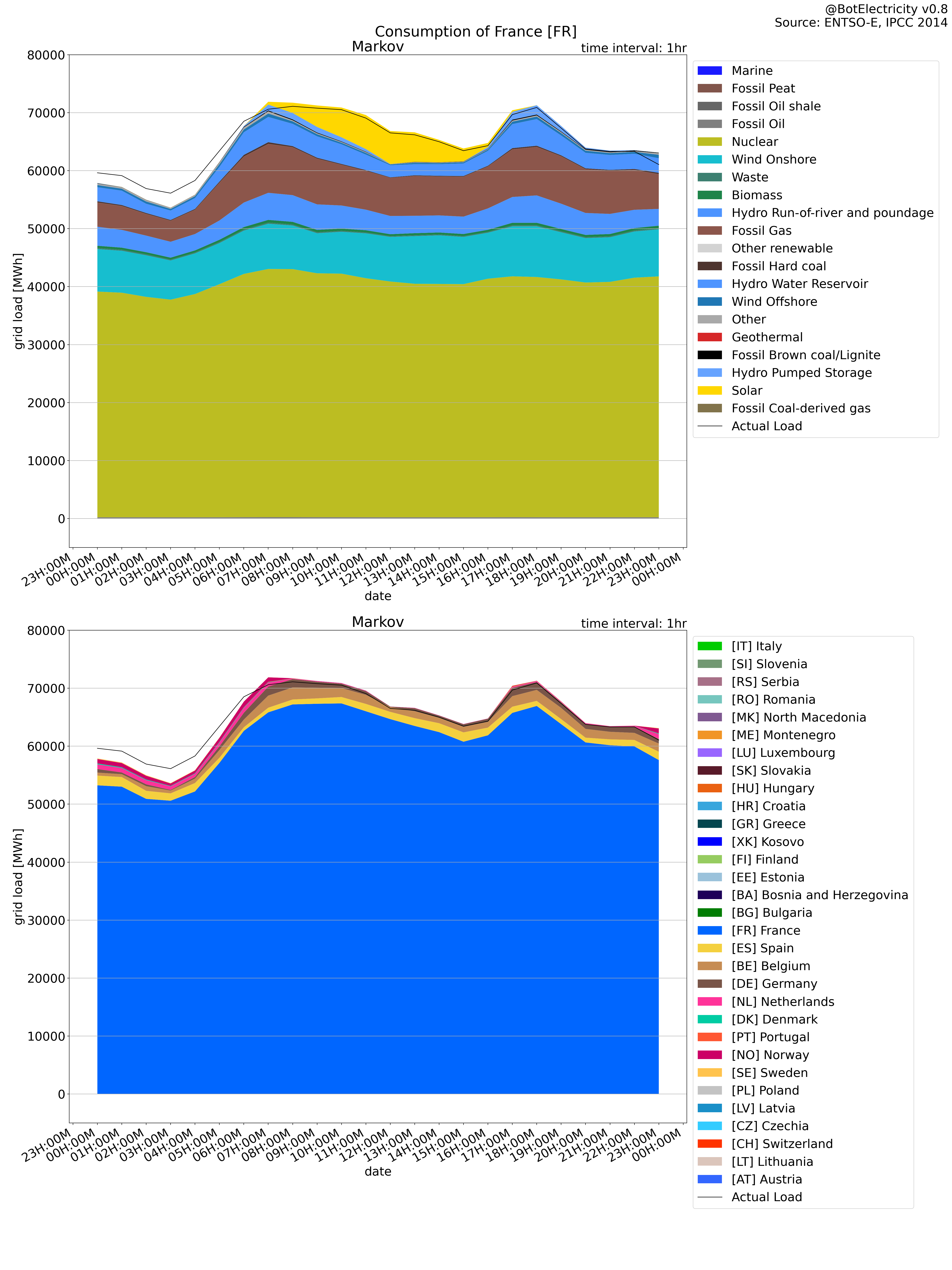
France present an interesting case. In the same day, it transitioned from a net importer to a net exporter. But it was still importing from a part of its neighbors.
The first two figures are the classic presentation with generation, storage and balance compared to the load.
Generation compared to production
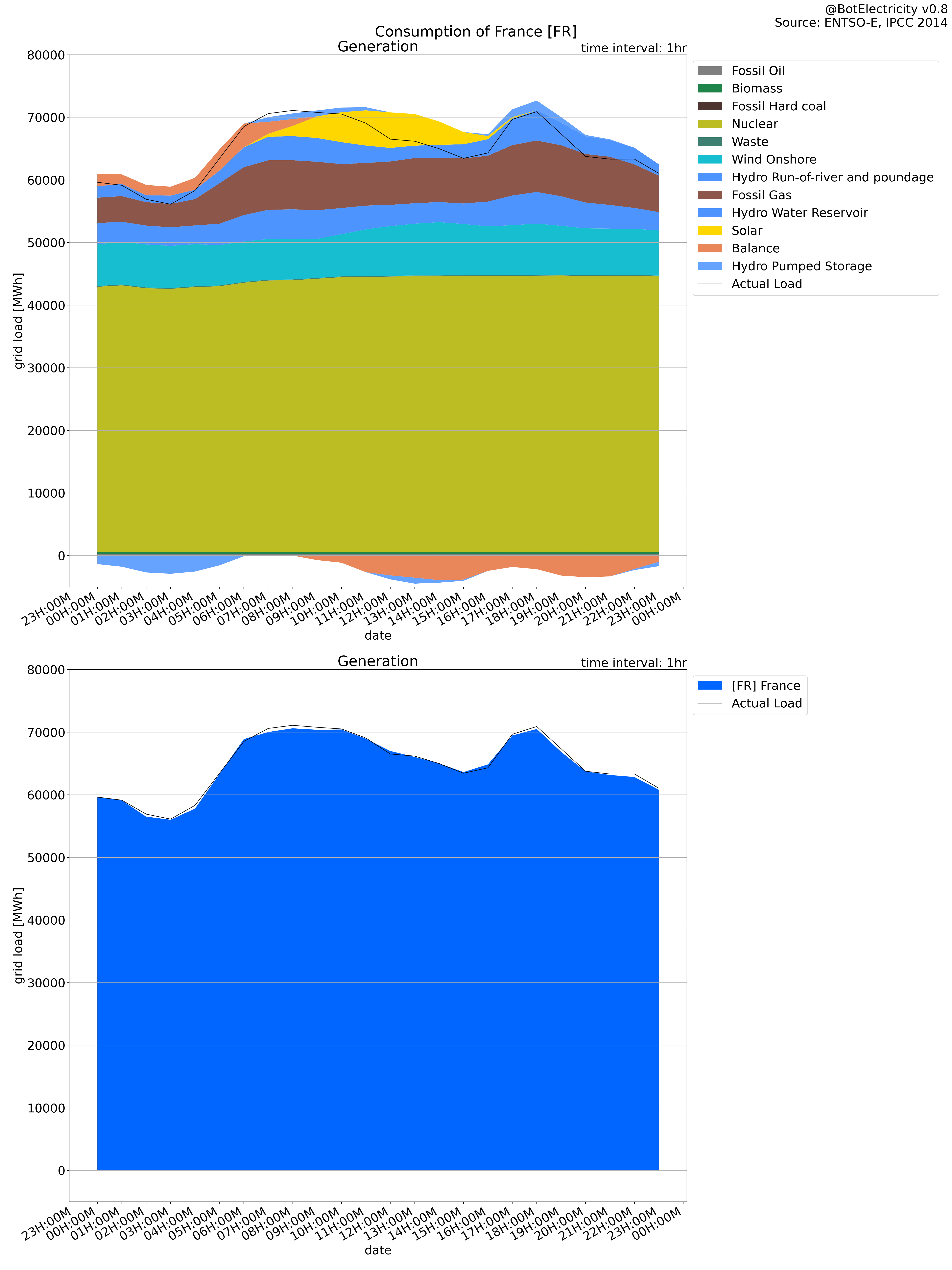
Markov production compared to consumption The Markov approach to define the consumption (where does the energy end) shows a total lower than the reported load.
Leontief load compared to load In the opposite, the Leontief approach match the load. However, the leontief is built in such a way that all the load is distributed.

Under the hood - Mathematical Approach
The mathematical tool used to compute the attribution is the solving of Markov chains for the production point of view and Leontief chain for the load point of view.
The graph must be a connected graph. The determinant of the graph is not zero.
From there it is possible to write equations. We will take the case of Portugal and Spain. There is a bit isolated from the European grid and it is easier to understand the idea. (There is the two countries on the top of the graph.)
To simplify the example, we assume there is only wind and coal as a source for both countries.
The energy entering the each country is:
Here we see France is implied. For this example we consider the France as unique source. We don't decompose it.
The energy leaving each country is:
It is not necessary to solve the equation analytically. There is the possibility to use matrices. We can call it the exchange matrix . For this, we assume the columns represent the energy provided and the rows the energy consumer.
Here is a simple example (without France).

| 0 | 0 | 0 | 0 | 0 | 0 | 0 | 0 | |
| 0 | 0 | 0 | 0 | 0 | 0 | 0 | 0 | |
| 0 | 0 | 0 | 0 | 0 | 0 | 0 | 0 | |
| 0 | 0 | 0 | 0 | 0 | 0 | 0 | 0 | |
| 300 | 200 | 0 | 0 | 0 | 250 | 0 | 0 | |
| 0 | 0 | 500 | 0 | 100 | 0 | 0 | 0 | |
| 0 | 0 | 0 | 0 | 650 | 0 | 0 | 0 | |
| 0 | 0 | 0 | 0 | 0 | 350 | 0 | 0 |
The import/export between countries is simplified as direct connection.
The matrix is then:
Depending on the studied case, a normalization operation is necessary:
- For the Markov approach, it is necessary to divide each row by its sum:
- For a Leontief approach, it is necessary to divide each column by its sum and apply a transposition:
Another vector will be necessary for to the operation: the result vector .
To solve the system we have to solve the equation:
is a matrix where the source are the columns and the rows the consumer. To check that there are no issues, it is possible to sum the lines and check it is similar to the complete vector.
With this method we have then a decomposition of the effect of the energy sources or consumption sink on each node of the graph.
In the previous example, the matrices are:
Compared to the previous table, this gives:
| Markov | ||||||||
| 300 | 0 | 0 | 0 | 0 | 0 | 0 | 0 | |
| 0 | 200 | 0 | 0 | 0 | 0 | 0 | 0 | |
| 0 | 0 | 500 | 0 | 0 | 0 | 0 | 0 | |
| 0 | 0 | 0 | 0 | 0 | 0 | 0 | 0 | |
| 218 | 212 | 221 | 0 | 0 | 0 | 0 | 0 | |
| 42 | 28 | 529 | 0 | 0 | 0 | 0 | 0 | |
| 275 | 184 | 191 | 0 | 0 | 0 | 0 | 0 | |
| 25 | 16 | 309 | 0 | 0 | 0 | 0 | 0 |
| Leontief | ||||||||
| 0 | 0 | 0 | 0 | 0 | 0 | 275 | 25 | |
| 0 | 0 | 0 | 0 | 0 | 0 | 184 | 16 | |
| 0 | 0 | 0 | 0 | 0 | 0 | 191 | 309 | |
| 0 | 0 | 0 | 0 | 0 | 0 | 0 | 0 | |
| 0 | 0 | 0 | 0 | 0 | 0 | 688 | 62 | |
| 0 | 0 | 0 | 0 | 0 | 0 | 299 | 371 | |
| 0 | 0 | 0 | 0 | 0 | 0 | 650 | 0 | |
| 0 | 0 | 0 | 0 | 0 | 0 | 0 | 350 |
Conclusion
As we conclude this exploration, it's clear that the task of estimating electricity consumption in an interconnected electrical grid is both complex and nuanced. The use of Markov and Leontief approaches has provided us with a specific view through which we can better understand the impact of the grid's nature on consumption patterns and provide an attribution of the flow of electricity from producers to consumers.
Through our case studies, we've seen how these mathematical models can illustrate the intricacies of electricity distribution, offering insights that are not immediately apparent through traditional methods. However, it's important to acknowledge the limitations and assumptions inherent in these models. The real-world application of these theories requires a careful consideration of these factors, along with a comprehensive understanding of the dynamic nature of electricity grids.
This article has only scratched the surface of what's possible with such mathematical tools. As the grid evolves with the integration of renewable energies and new technologies, new behaviors on the grid can be observed. For instance, it is possible to study the source of energy from one country and see where it propagates and where the bottlenecks are. Indeed, even if the interconnections are sufficients, it is possible that several power sources enter into competition to cross such an interconnection. The pursuit of a more efficient, reliable, and sustainable electricity grid continues, and it is our hope that the methodologies discussed here will contribute to this ongoing evolution.
The code to generate the figures is available in this file.